Plot the weights for an observation

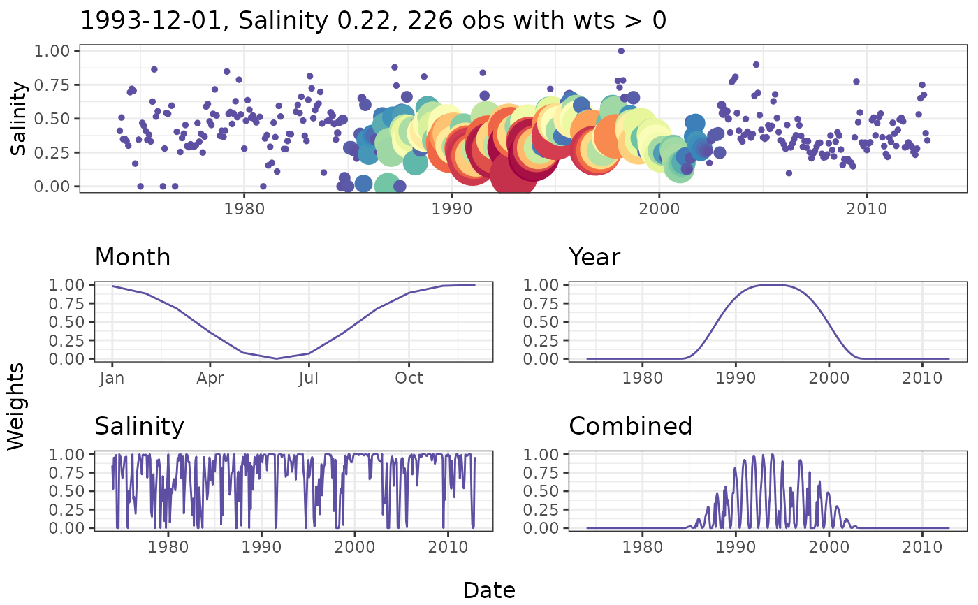
Create several plots showing the weights used to fit a model for a single observation.

wtsplot(dat_in, ...)

# S3 method for default
wtsplot(
  dat_in,
  ref = NULL,
  wins = list(0.5, 10, NULL),
  min_obs = TRUE,
  slice = FALSE,
  dt_rng = NULL,
  pt_rng = c(1, 12),
  col_vec = NULL,
  col_lns = NULL,
  alpha = 1,
  as_list = FALSE,
  ...
)

# S3 method for tidal
wtsplot(dat_in, ...)

# S3 method for tidalmean
wtsplot(dat_in, ...)

Arguments

dat_in

input tidal object

...

arguments passed to other methods

ref

chr string indicating the date at the center of the weighting window. Must be in the format 'YYYY-mm-dd' which is passed to as.Date. The closest observation is used if the actual is not present in the data. Defaults to the mean date if not supplied.

wins

list with three elements passed to getwts indicating the half-window widths for day, year, and salinity/flow

min_obs

logical to use window widening if less than 100 non-zero weights are found, passed to getwts

slice

logical indicating if only weights bounded by the year window (i.e., the limiting window for the combined weights) are shown, passed to getwts

dt_rng

Optional chr string indicating the date range for all plots except seasonal (day) weights. Must be two values in the format 'YYYY-mm-dd' which is passed to as.Date.

pt_rng

numeric vector of two elements indicating point scaling for all weights in the plot of salinity/flow vs time.

col_vec

chr string of plot colors to use, passed to gradcols and scale_colour_gradientn for weight shading. The last value in the vector is used as the line color if col_lns = NULL. Any color palette from RColorBrewer can be used as a named input. Palettes from grDevices must be supplied as the returned string of colors for each palette.

col_lns

chr string of line color in plots

alpha

numeric value from zero to one indicating transparency of points and lines

as_list

logical indicating if plots should be returned in a list

Value

A combined ggplot object created using grid.arrange. A list with elements for each individual plot will be returned if as_list = TRUE.

Details

Create diagnostic plots to view the effects of different weighting windows on model predictions. The plots illustrate the weights that are used when fitting a weighted regression in reference to a single observation. The process is repeated for all observations when the entire model is fit. Five plots are produced by the function, each showing the weights in relation to time and the selected observation (i.e., center of the weighting window). The top plot shows salinity/flow over time with the points colored and sized by the combined weight vector. The remaining four plots show the weights over time for each separate weighting component (months/days, year, and salinity/flow) and the final combined vector.

See also

getwts

Examples

## load a fitted tidal object
data(tidfit)

## plot using defaults, 
wtsplot(tidfit)


## change the defaults
wtsplot(tidfit, ref = '2000-01-01', wins = list(0.5, 15, Inf), 
 dt_rng = c('1990-01-01', '2010-01-01'), 
 pt_rng = c(3, 8), col_vec = c('lightgreen', 'lightblue', 'purple'),
 alpha = 0.7)
#> Warning: Removed 211 rows containing missing values (`geom_line()`).
#> Warning: Removed 211 rows containing missing values (`geom_line()`).
#> Warning: Removed 211 rows containing missing values (`geom_line()`).
#> Warning: Removed 211 rows containing missing values (`geom_point()`).