EBASE sensitivity analysis
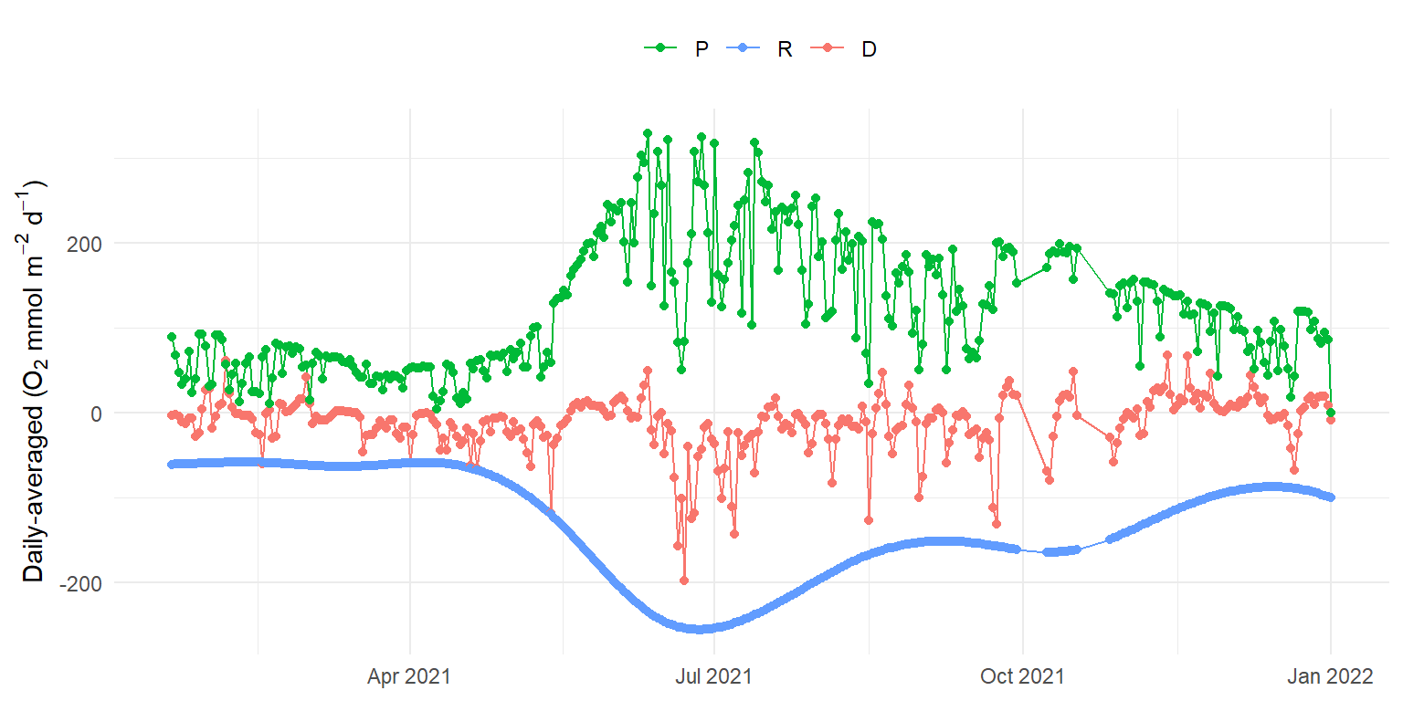
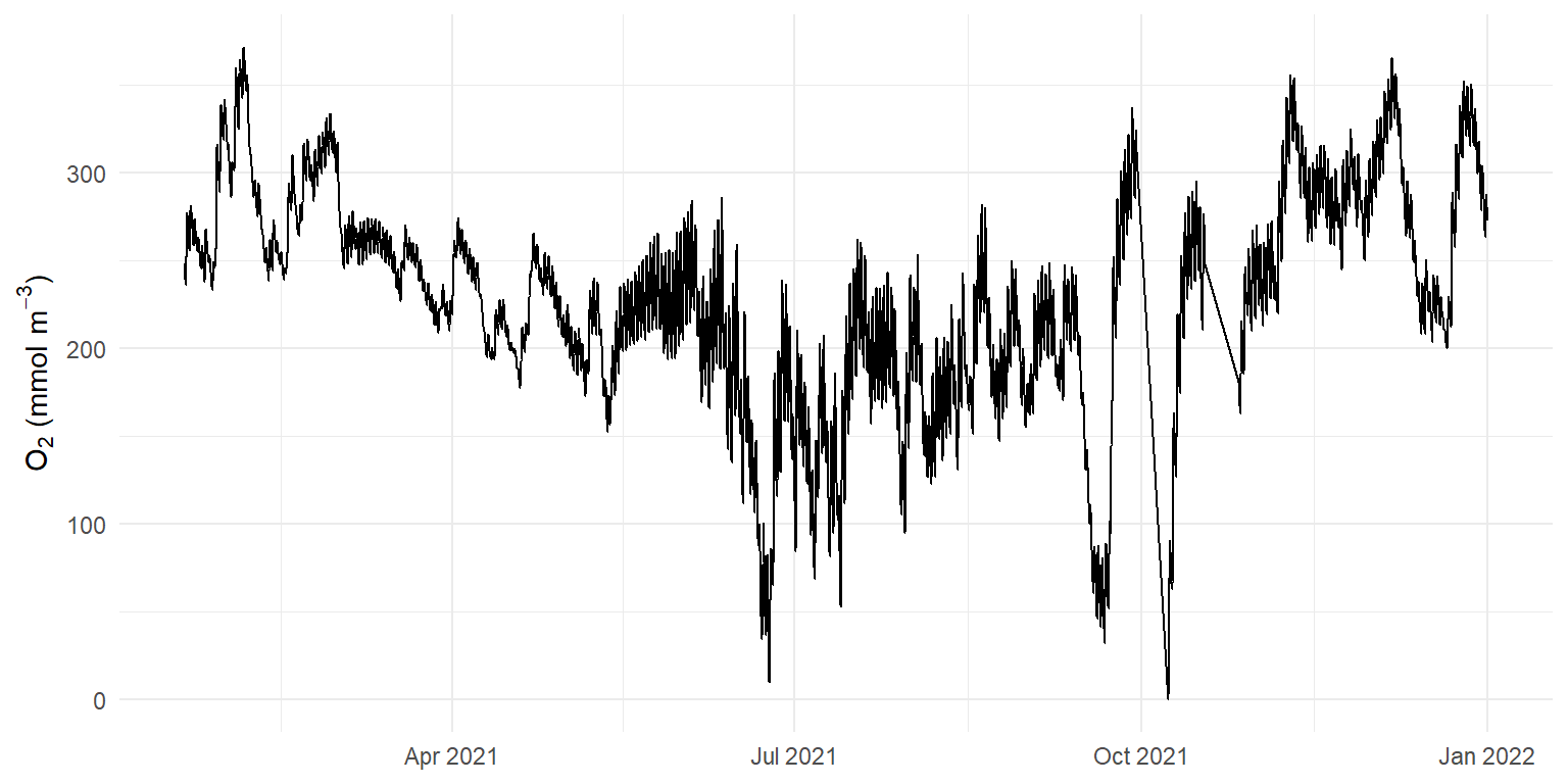
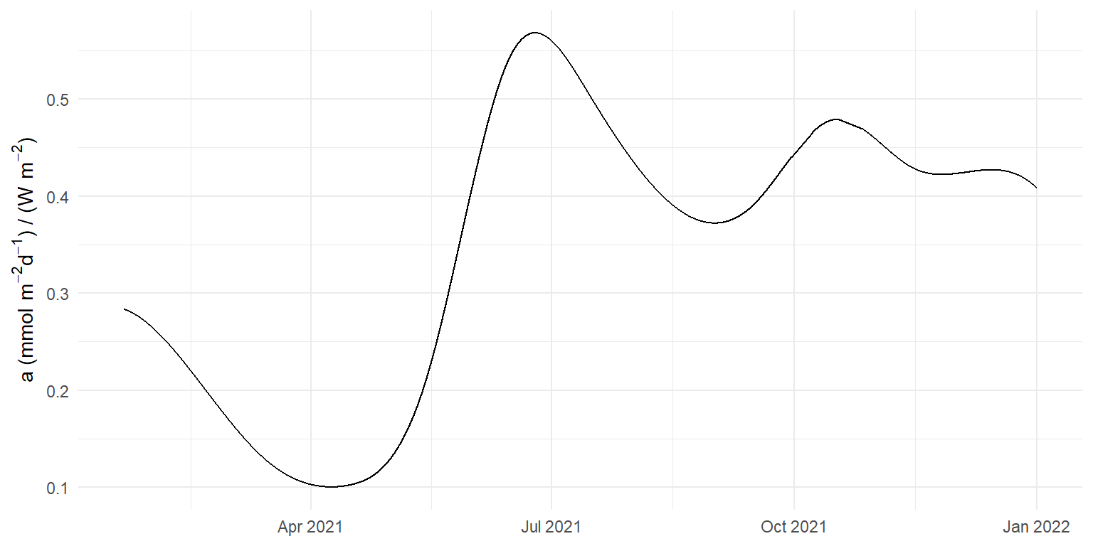
This page describes a sensitivity analysis of EBASE to estimate metabolic rates and parameters using a time series with known inputs. The known time series used field-derived data from Apalachicola Bay to simulate data using a forward oxygen mass balance model from Fwoxy.
The sensitivity analysis included two separate evaluations. The first evaluated three different prior distributions that assessed changes in the standad deviation for the \(a\), \(r\), and \(b\) parameters in the equation below. The second evaluated three different prior distributions for the \(b\) parameter only Model optimization periods were also compared using one and seven days for each combination of prior distributions.
\[ \frac{\delta{C_d}}{\delta{t}} = [\,aPAR]\, - [\,r]\, - \frac{1}{H}\left[-bU_{10}^2\left(\frac{s_c}{600} \right)^{-0.5} \left(C_{Sat} - C_d \right )\right] \]
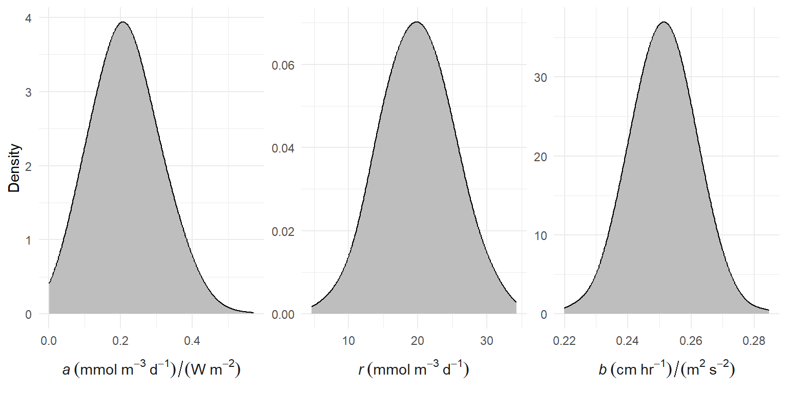
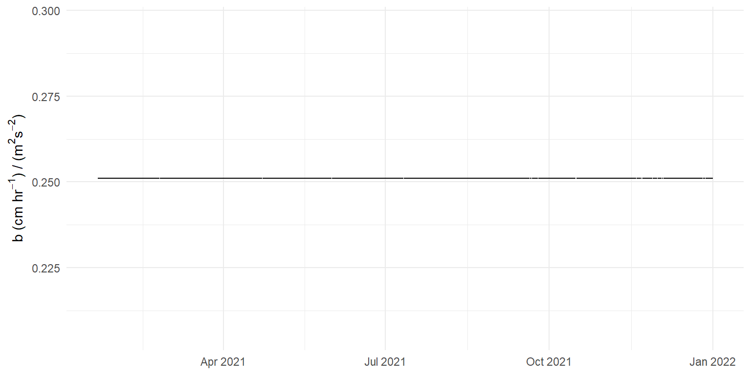
The default prior distributions for EBASE are as follows, where the standard deviations for \(a\), \(r\), and \(b\) are 0.1, 5, and 0.01:
Analysis 1
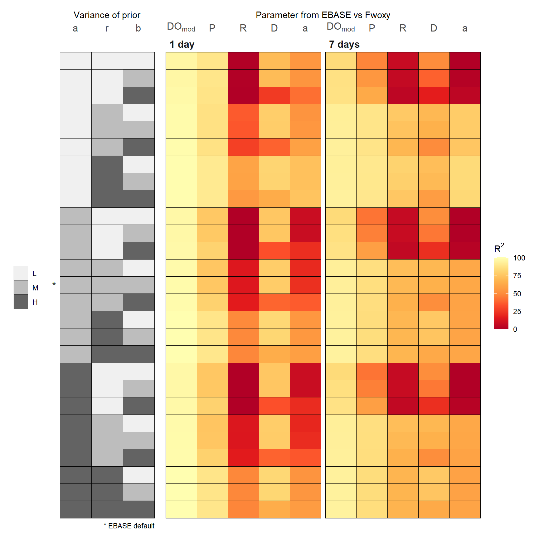
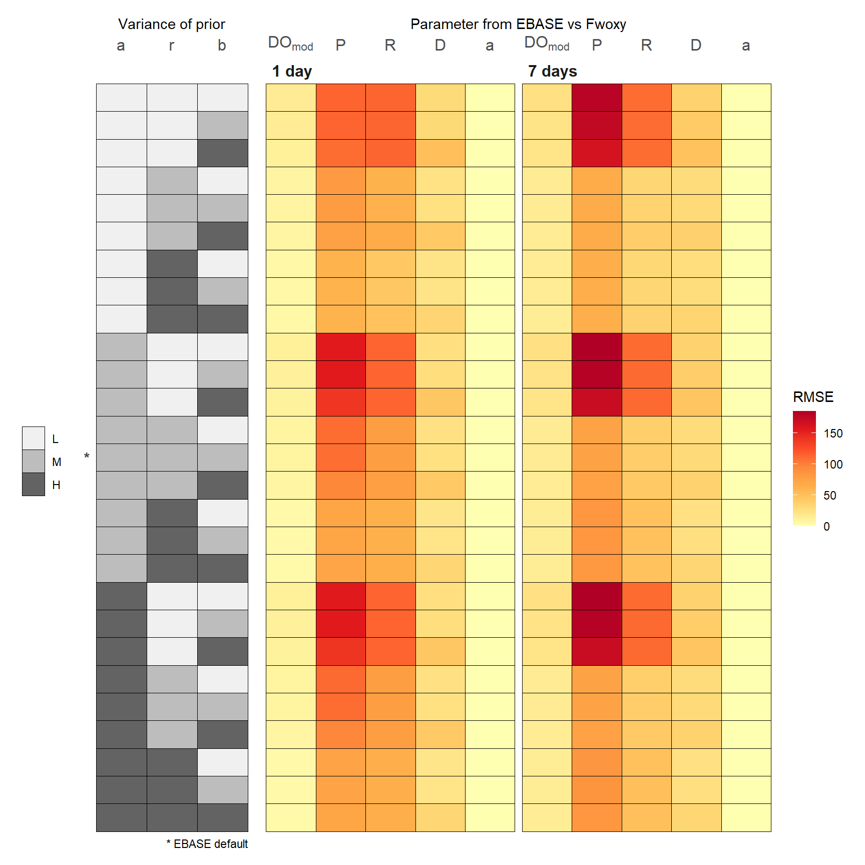
Each prior distribution was varied for \(a\), \(r\), and \(b\) by using a different standard deviation from small to large to test the effect of more or less constrained ranges, respectively, on the priors. A total of 54 combinations for each of two optimization periods were evaluated, where the “low”, “medium”, or “high” ranges on the standard deviations for the priors varied by orders of magnitude (10%, 100% [default], and 1000%) from the default values. Any prior indicating “M” is the default value.
| a (sd) | r (sd) | b (sd) |
|---|---|---|
| 0.01 (L) | 0.5 (L) | 0.001 (L) |
| 0.01 (L) | 0.5 (L) | 0.01 (M) |
| 0.01 (L) | 0.5 (L) | 0.1 (H) |
| 0.01 (L) | 5 (M) | 0.001 (L) |
| 0.01 (L) | 5 (M) | 0.01 (M) |
| 0.01 (L) | 5 (M) | 0.1 (H) |
| 0.01 (L) | 50 (H) | 0.001 (L) |
| 0.01 (L) | 50 (H) | 0.01 (M) |
| 0.01 (L) | 50 (H) | 0.1 (H) |
| 0.1 (M) | 0.5 (L) | 0.001 (L) |
| 0.1 (M) | 0.5 (L) | 0.01 (M) |
| 0.1 (M) | 0.5 (L) | 0.1 (H) |
| 0.1 (M) | 5 (M) | 0.001 (L) |
| 0.1 (M) | 5 (M) | 0.01 (M) |
| 0.1 (M) | 5 (M) | 0.1 (H) |
| 0.1 (M) | 50 (H) | 0.001 (L) |
| 0.1 (M) | 50 (H) | 0.01 (M) |
| 0.1 (M) | 50 (H) | 0.1 (H) |
| 1 (H) | 0.5 (L) | 0.001 (L) |
| 1 (H) | 0.5 (L) | 0.01 (M) |
| 1 (H) | 0.5 (L) | 0.1 (H) |
| 1 (H) | 5 (M) | 0.001 (L) |
| 1 (H) | 5 (M) | 0.01 (M) |
| 1 (H) | 5 (M) | 0.1 (H) |
| 1 (H) | 50 (H) | 0.001 (L) |
| 1 (H) | 50 (H) | 0.01 (M) |
| 1 (H) | 50 (H) | 0.1 (H) |
Analysis 2
The prior distribution for only the \(b\) parameter was varied by changing both the mean and standard deviation values. This additional analysis was done to determine if the fixed \(b\) parameter could be recovered with priors that are outside of the range of the actual value. Nine combinations were evaluated based on three different values for the mean (50% of the default, default, and 200% of the default) and three different values for the standard deviation (10% of the default, default, and 1000% of the default). The default values in EBASE for the prior distributions of \(a\) and \(r\) were used. As before, one day and seven day optimization periods were also evaluated.
| b (mean) | b (sd) |
|---|---|
| 0.1255 (L) | 0.001 (L) |
| 0.1255 (L) | 0.01 (M) |
| 0.1255 (L) | 0.1 (H) |
| 0.251 (M) | 0.001 (L) |
| 0.251 (M) | 0.01 (M) |
| 0.251 (M) | 0.1 (H) |
| 0.502 (H) | 0.001 (L) |
| 0.502 (H) | 0.01 (M) |
| 0.502 (H) | 0.1 (H) |
Evaluating the output
The output from EBASE for each analysis and combination of prior distributions was compared to the known values from the simulated time series. Note that the \(b\) parameter is fixed and estimated from \(k_w\), \(U^2_{10}\), and \(s_c\).
Analysis 1
The following shows a summary of the model output for each unique combination of prior distributions and two optimization periods of one and seven days for the simulated time series. The comparisons show the difference, evaluated as R\(^2\) or RMSE, for each parameter from EBASE relative to those from Fwoxy. Note that the \(b\) parameter is not evaluated because it is constant throughout the time series and parameters that are returned as a single estimate for the optimization period of the model were compared to the average parameter from Fwoxy for the same optimization period. The latter applies to \(Rt_{vol}\) and \(a\). Warmer colors indicate lower R\(^2\) and higher RMSE, or reduced similarities.
R-squared
RMSE
Analysis 2
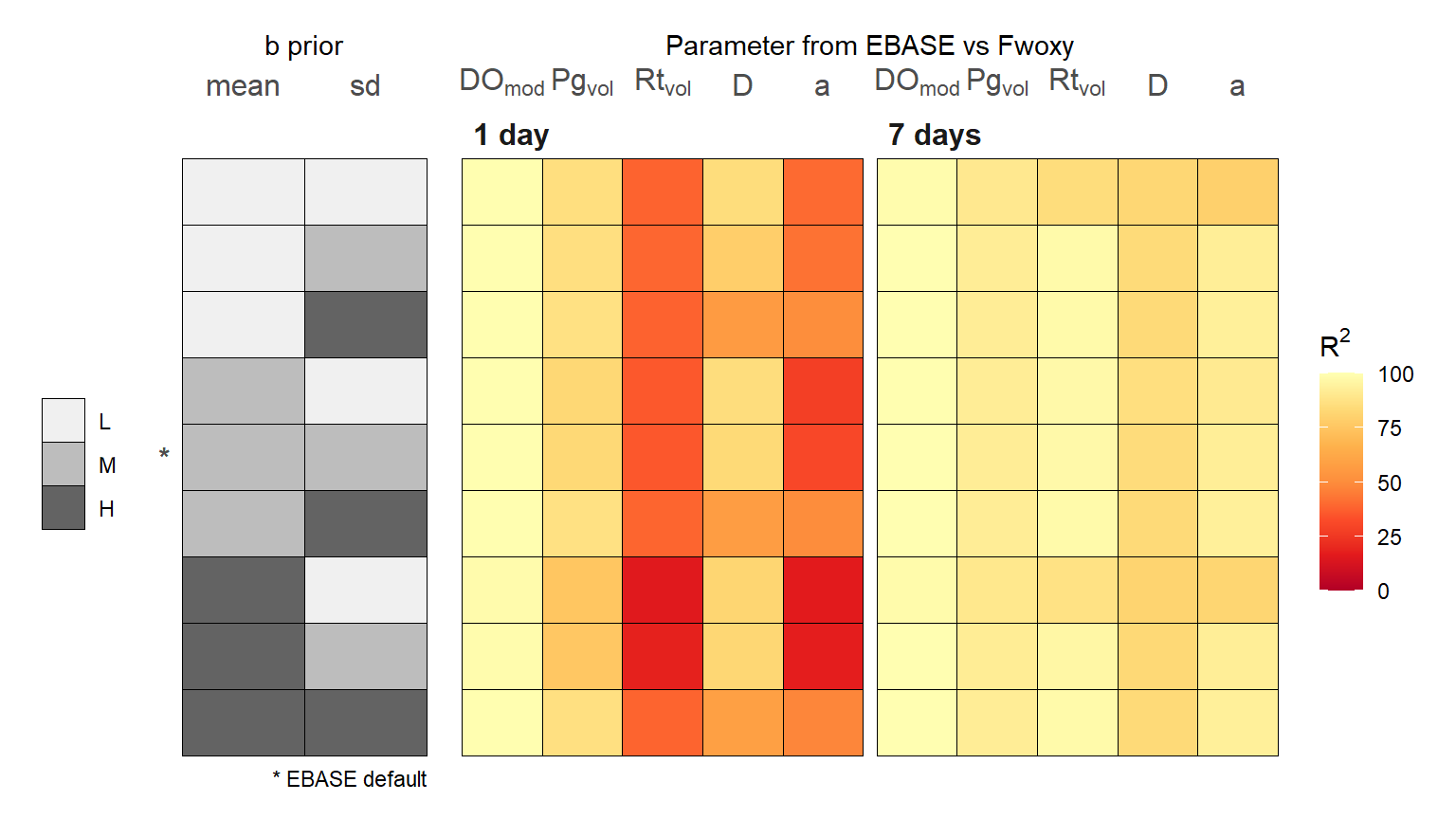
R-squared
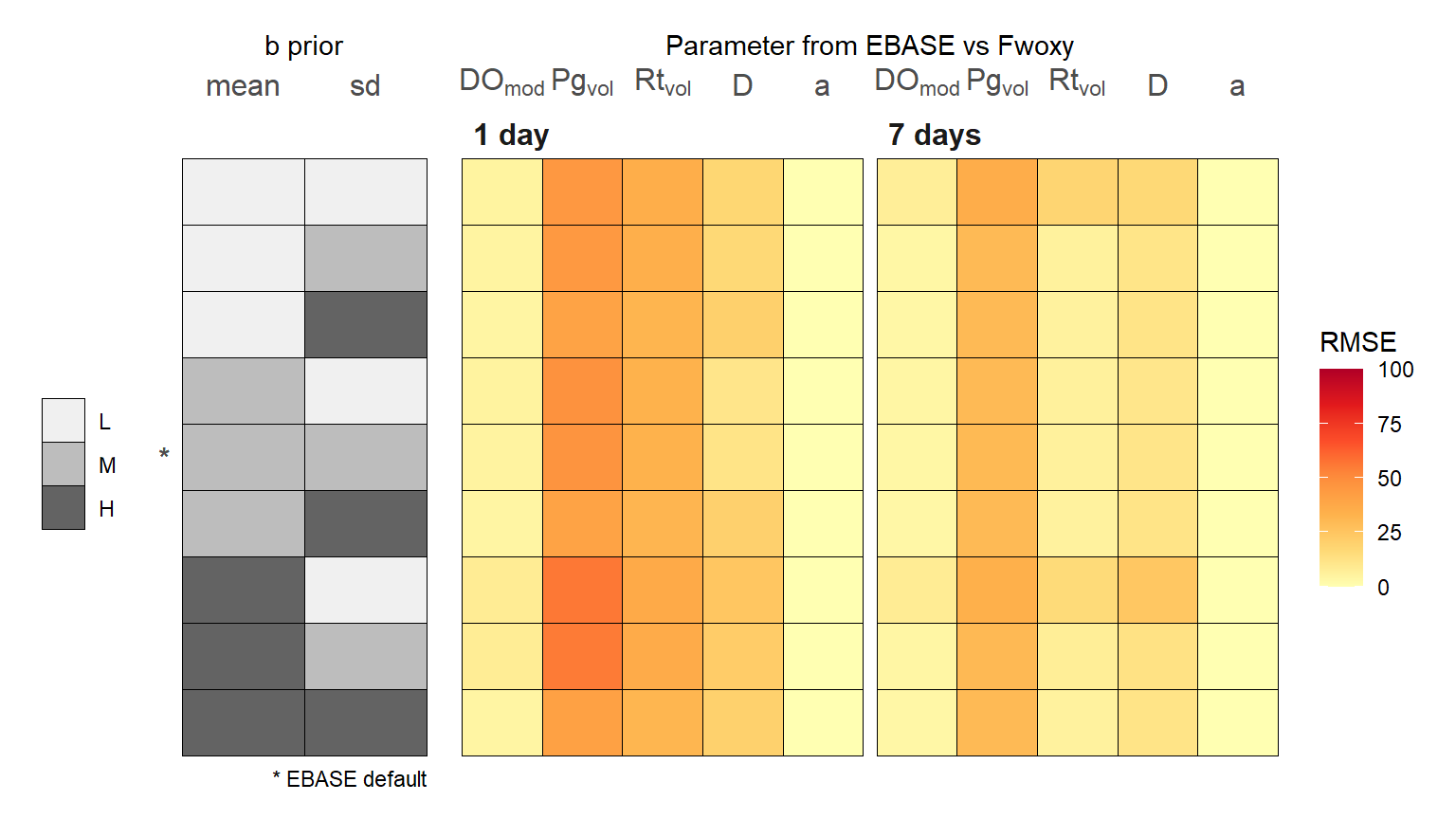
RMSE
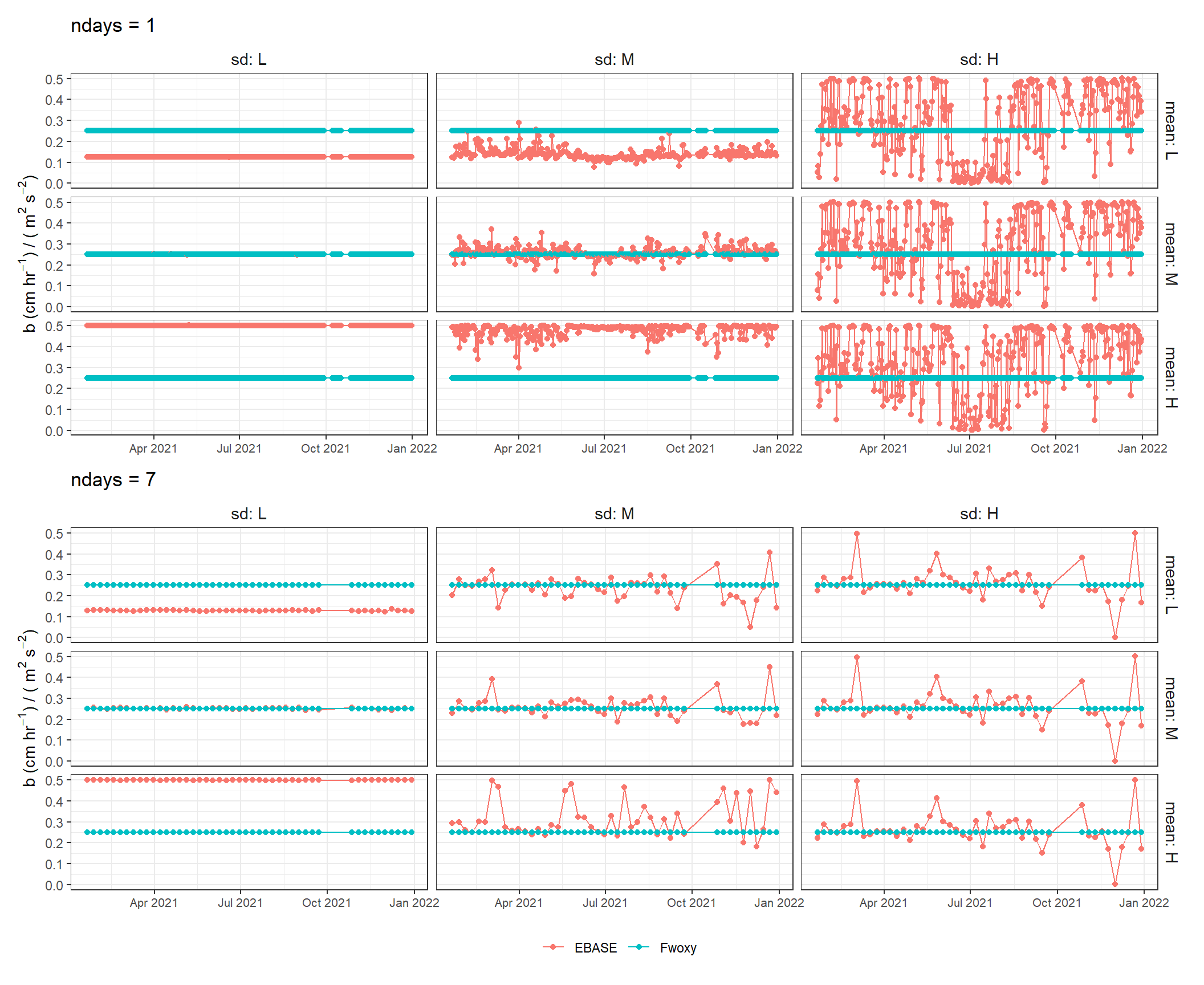
b only
A summary of the \(b\) parameter for different priors for each time step and optimization period.
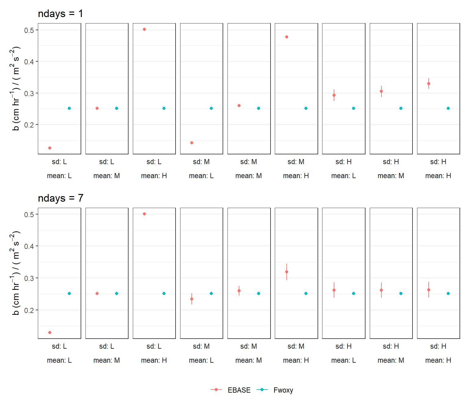
Same results as above, but \(b\) is summarized as the average and 95% confidence interval across the time series for each prior combination.
Analysis 1
Several conclusions can be made from the sensitivity analysis regarding the ability of EBASE to estimate the known parameters from the simulated Fwoxy time series. These are based on identified patterns in the R\(^2\) and RMSE estimates for different combinations of the priors.
- Parameter estimates for \(a\) are minimally influenced by changes in the variance of the priors
- Lower variance of the \(r\) prior distribution contributed to lower R\(^2\) and higher RMSE values for all parameters, the fit was worse with a longer optimization period (e.g, lower R\(^2\) for the \(a\) parameter and higher RMSE for Pg\(_{vol}\) at seven day optimization)
- Higher variance of the \(b\) prior distribution contributed to lower R\(^2\) and higher RMSE values for most parameters (e.g., lower R\(^2\) and higher RMSE for D)
- Longer optimization period generally improved fits in parameter estimates, with some exceptions noted above
Recommendation:
- The default prior distributions for the parameters may be appropriate in some cases, but increasing the variance for \(a\) and \(r\) and decreasing the variance for \(b\) produces more optimal solutions. The top three optimal solutions based on maximum average R\(^2\) or minimum average RMSE are as follows for each optimization period, where the top three combinations for each are shown below.
| a (sd) | r (sd) | b (sd) | ndays | Ave. R2 | Ave. RMSE | R2 rank | RMSE rank |
|---|---|---|---|---|---|---|---|
| 0.01 (L) | 50 (H) | 0.001 (L) | 1 | 67.41273 | 22.19603 | 1 | 1 |
| 0.01 (L) | 50 (H) | 0.01 (M) | 1 | 67.33303 | 22.27657 | 2 | 2 |
| 0.01 (L) | 50 (H) | 0.1 (H) | 1 | 63.85183 | 24.96941 | 3 | 3 |
| 0.01 (L) | 5 (M) | 0.001 (L) | 7 | 67.51366 | 24.03514 | 3 | 3 |
| 0.01 (L) | 50 (H) | 0.001 (L) | 7 | 69.96137 | 23.15619 | 1 | 1 |
| 0.01 (L) | 50 (H) | 0.01 (M) | 7 | 69.52616 | 23.54911 | 2 | 2 |
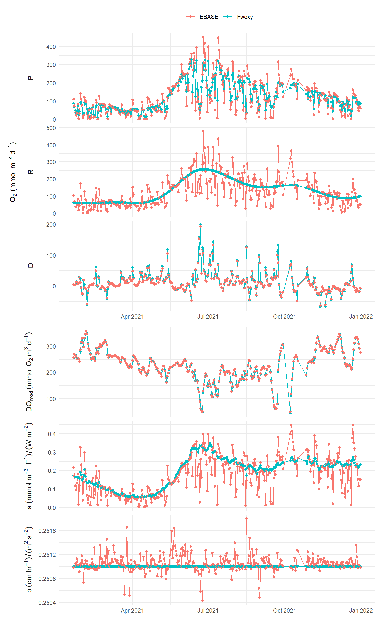
Result comparisons at the time step of the optimization period are shown for different examples of the optimal prior distributions from above.
a (sd) = 1, r (sd) = 50, b (sd) = 0.001, ndays = 1
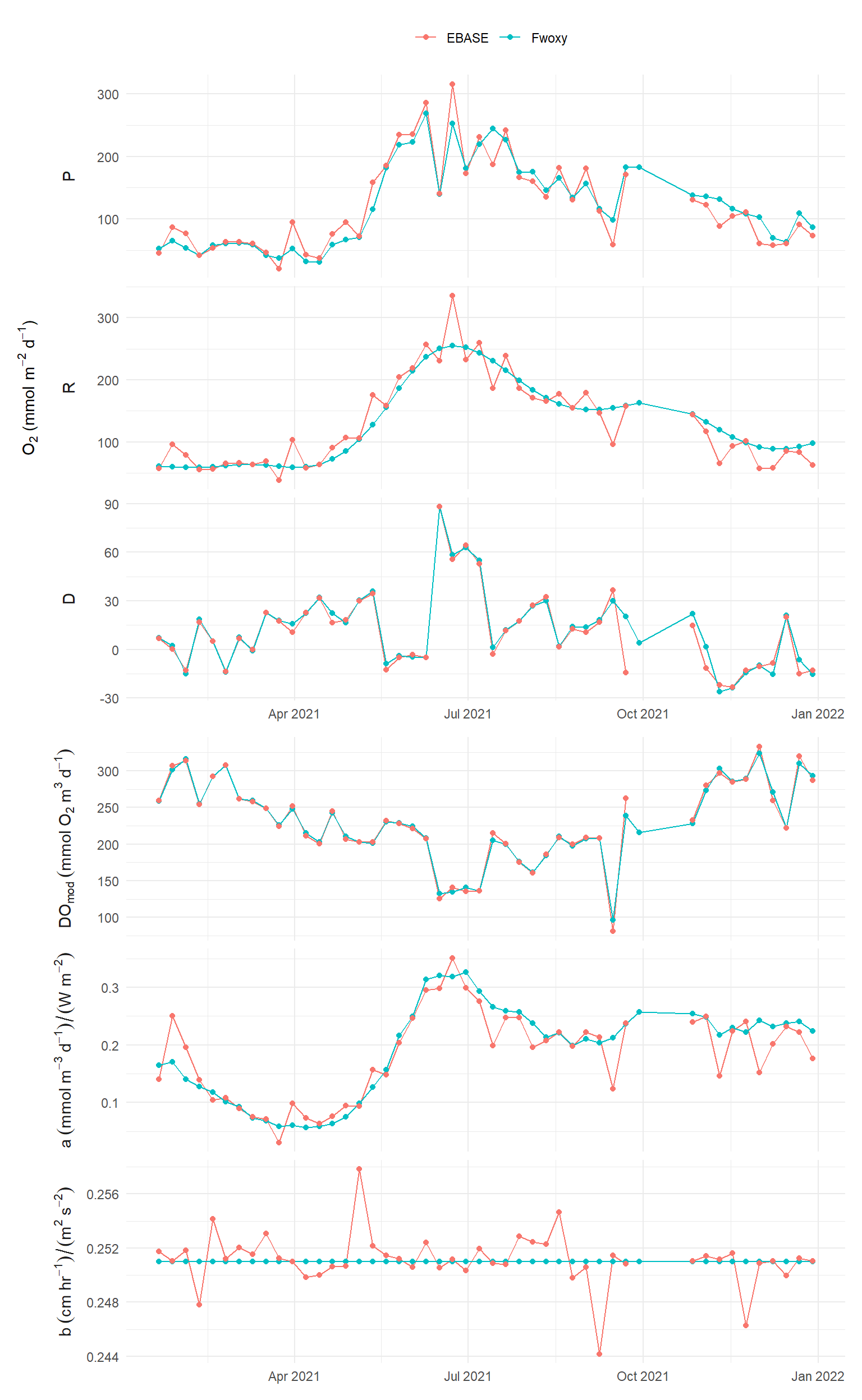
a (sd) = 0.01, r (sd) = 50, b (sd) = 0.001, ndays = 7
Analysis 2
Higher values for the mean of the \(b\) prior distribution parameter generally produce less precise parameter estimates, especally for \(Rt_{vol}\) and \(a\). This effect is mitigated with a larger value for the standard deviation of the prior distribution. All of these issues are negligible for a longer optimization period.
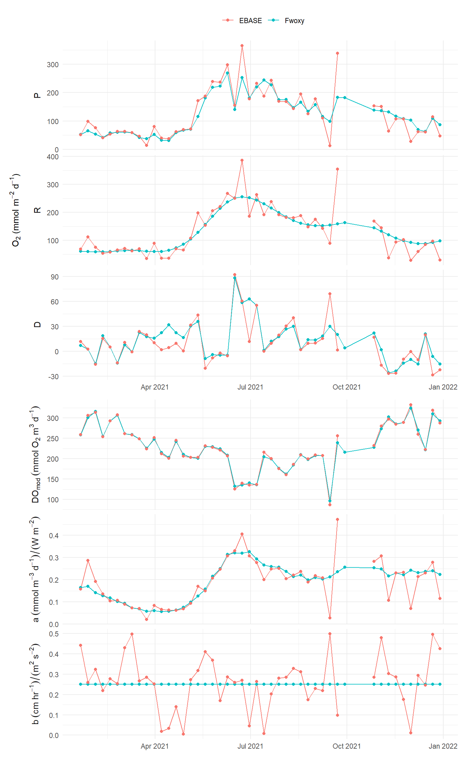
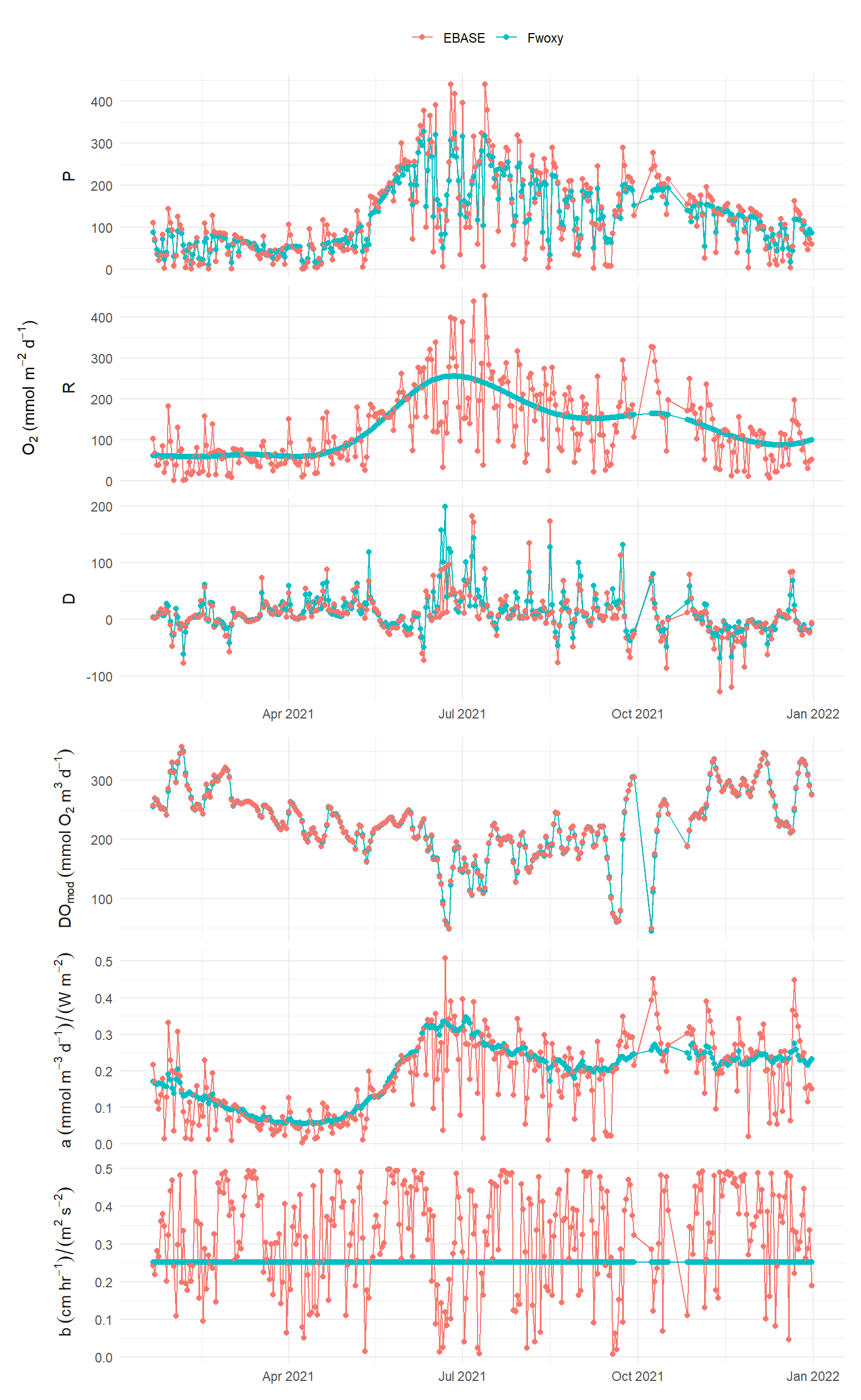
For fun, here’s what the model results for EBASE look like compared to Fwoxy using very uninformed priors (high standard deviation for all).
a (sd) = 1, r (sd) = 50, b (sd) = 0.1, ndays = 1
a (sd) = 1, r (sd) = 50, b (sd) = 0.1, ndays = 7