Plot a neural network model — plotnet • NeuralNetTools

Plot a neural interpretation diagram for a neural network object

plotnet(mod_in, ...)

# S3 method for default
plotnet(
  mod_in,
  x_names,
  y_names,
  struct = NULL,
  nid = TRUE,
  all_out = TRUE,
  all_in = TRUE,
  bias = TRUE,
  bias_y = 0.95,
  rel_rsc = c(1, 7),
  circle_cex = 5,
  node_labs = TRUE,
  var_labs = TRUE,
  line_stag = NULL,
  cex_val = 1,
  alpha_val = 1,
  circle_col = "lightblue",
  pos_col = "black",
  neg_col = "grey",
  bord_col = "lightblue",
  max_sp = FALSE,
  pad_x = 1,
  prune_col = NULL,
  prune_lty = "dashed",
  skip = NULL,
  ...
)

# S3 method for nnet
plotnet(mod_in, x_names = NULL, y_names = NULL, skip = FALSE, ...)

# S3 method for numeric
plotnet(mod_in, struct, x_names = NULL, y_names = NULL, ...)

# S3 method for mlp
plotnet(
  mod_in,
  x_names = NULL,
  y_names = NULL,
  prune_col = NULL,
  prune_lty = "dashed",
  ...
)

# S3 method for nn
plotnet(mod_in, x_names = NULL, y_names = NULL, ...)

# S3 method for train
plotnet(mod_in, x_names = NULL, y_names = NULL, skip = FALSE, ...)

Arguments

mod_in: neural network object or numeric vector of weights
...: additional arguments passed to or from other methods
x_names: chr string indicating names for input variables, default from model object
y_names: chr string indicating names for output variables, default from model object
struct: numeric vector equal in length to the number of layers in the network. Each number indicates the number of nodes in each layer starting with the input and ending with the output. An arbitrary number of hidden layers can be included.
nid: logical value indicating if neural interpretation diagram is plotted, default TRUE
all_out: chr string indicating names of response variables for which connections are plotted, default all
all_in: chr string indicating names of input variables for which connections are plotted, default all
bias: logical value indicating if bias nodes and connections are plotted, default TRUE
bias_y: value from 0 to 1 for locattion of bias nodes on y-axis
rel_rsc: numeric indicating the scaling range for the width of connection weights
circle_cex: numeric value indicating size of nodes, default 5
node_labs: logical value indicating if labels are plotted directly on nodes, default TRUE
var_labs: logical value indicating if variable names are plotted next to nodes, default TRUE
line_stag: numeric value that specifies distance of connection weights from nodes
cex_val: numeric value indicating size of text labels, default 1
alpha_val: numeric value (0-1) indicating transparency of connections, default 1
circle_col: chr string indicating color of nodes, default 'lightblue', or two element list with first element indicating color of input nodes and second indicating color of remaining nodes
pos_col: chr string indicating color of positive connection weights, default 'black'
neg_col: chr string indicating color of negative connection weights, default 'grey'
bord_col: chr string indicating border color around nodes, default 'lightblue'
max_sp: logical value indicating if space between nodes in each layer is maximized, default FALSE
pad_x: numeric for increasing or decreasing padding on the x-axis, values less than one will increase padding and values greater than one will decrease padding
prune_col: chr string indicating color of pruned connections, otherwise not shown
prune_lty: line type for pruned connections, passed to segments
skip: logical if skip layer connections are plotted instead of the primary network

Value

A graphics object unless wts_only = TRUE, then neural network weights from neuralweights.

Details

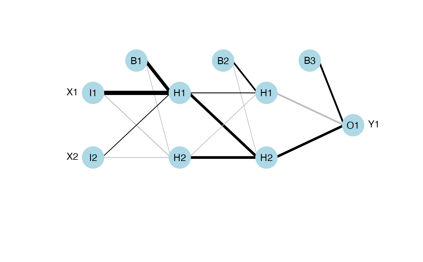
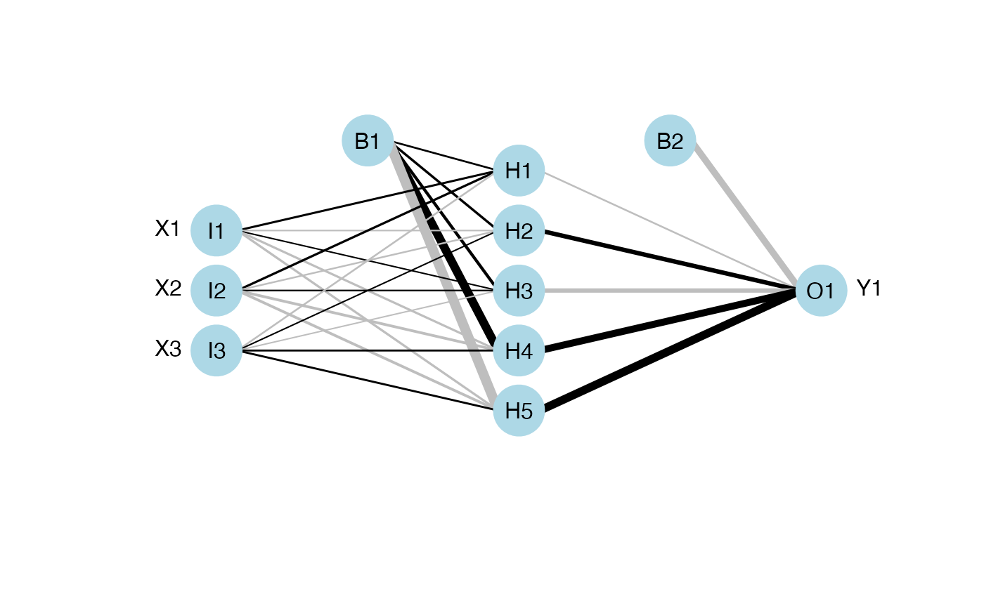
This function plots a neural network as a neural interpretation diagram as in Ozesmi and Ozesmi (1999). Options to plot without color-coding or shading of weights are also provided. The default settings plot positive weights between layers as black lines and negative weights as grey lines. Line thickness is in proportion to relative magnitude of each weight. The first layer includes only input variables with nodes labelled arbitrarily as I1 through In for n input variables. One through many hidden layers are plotted with each node in each layer labelled as H1 through Hn. The output layer is plotted last with nodes labeled as O1 through On. Bias nodes connected to the hidden and output layers are also shown. Neural networks created using mlp do not show bias layers.

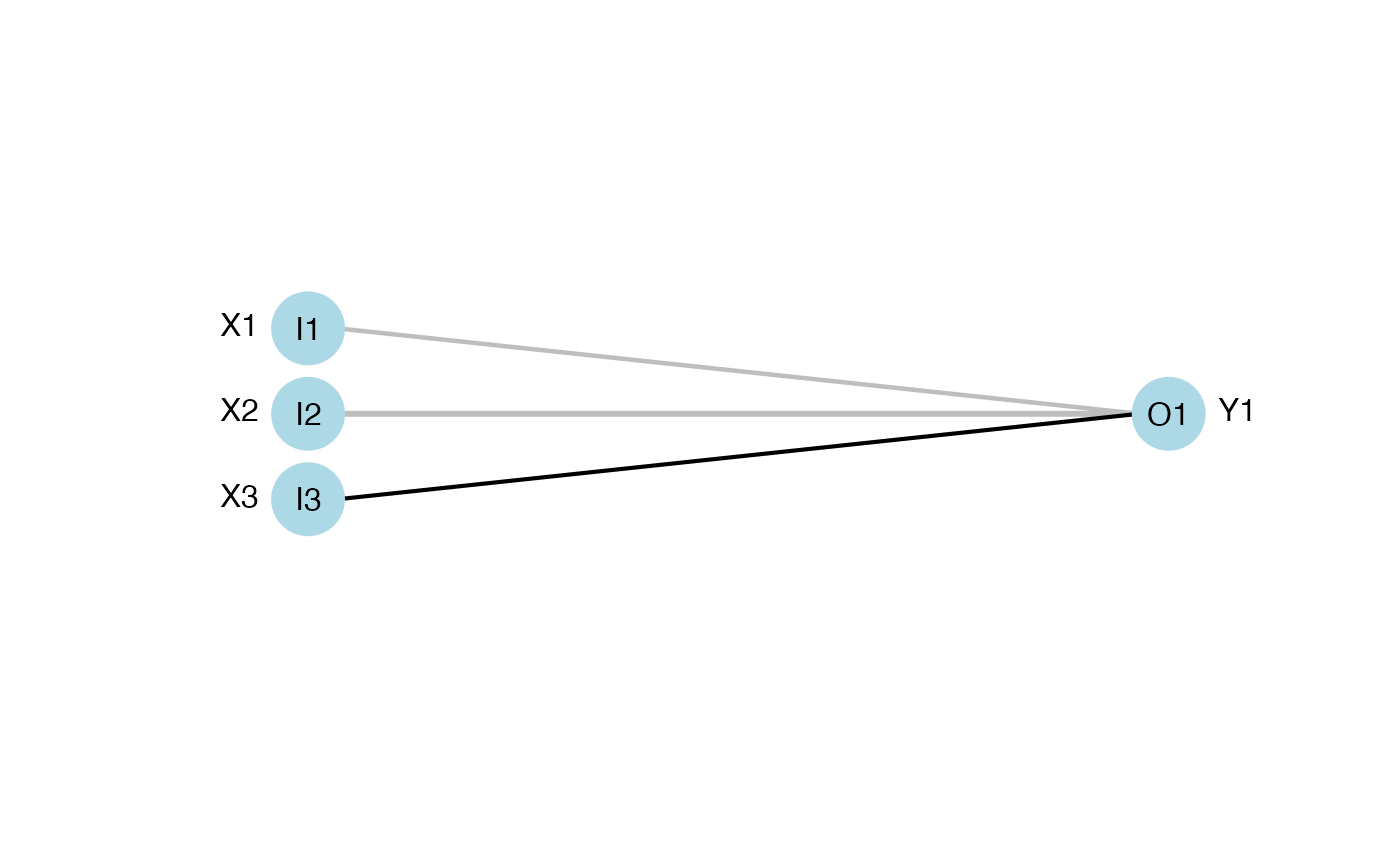
A primary network and a skip layer network can be plotted for nnet models with a skip layer connection. The default is to plot the primary network, whereas the skip layer network can be viewed with skip = TRUE. If nid = TRUE, the line widths for both the primary and skip layer plots are relative to all weights. Viewing both plots is recommended to see which network has larger relative weights. Plotting a network with only a skip layer (i.e., no hidden layer, size = 0) will include bias connections to the output layer, whereas these are not included in the plot of the skip layer if size is greater than zero.

The numeric method for plotting requires the input weights to be in a specific order given the structure of the network. An additional argument struct (from neuralweights is also required that lists the number of nodes in the input, hidden, and output layers. The example below for the numeric input shows the correct weight vector for a simple neural network model with two input variables, one output variable, and one hidden layer with two nodes. Bias nodes are also connected to the hidden and output layer. Using the plot syntax of I, H, O, and B for input, hidden, output, and bias to indicate weighted connections between layers, the correct weight order for the mod_in vector is B1-H1, I1-H1, I2-H1, B1-H2, I1-H2, I2-H2, B2-O1, H1-O1, H2-O1. For a generic network (three layers) with n input nodes, j hidden nodes, and k output nodes, the weights are ordered as the connections from B1, I1,...,In to H1,...,Hj, then B2, H1,..,Hj to O1,...,Ok.

References

Beck, M.W. 2018. NeuralNetTools: Visualization and Analysis Tools for Neural Networks. Journal of Statistical Software. 85(11):1-20.

Ozesmi, S.L., Ozesmi, U. 1999. An artificial neural network approach to spatial habitat modeling with interspecific interaction. Ecological Modelling. 116:15-31.

Examples

## using numeric input

# B1-H1, I1-H1, I2-H1, B1-H2, I1-H2, I2-H2, B2-O1, H1-O1, H2-O1.
wts_in <- c(13.12, 1.49, 0.16, -0.11, -0.19, -0.16, 0.56, -0.52, 0.81)
struct <- c(2, 2, 1) #two inputs, two hidden, one output 

plotnet(wts_in, struct = struct)


# numeric input, two hidden layers

# B1-H11, I1-H11, I2-H11, B1-H12, I1-H12, I2-H12, B2-H21, H11-H21, H12-H21, 
# B2-H22, H11-H22, H12-H22, B3-O1, H21-O1, H22-O1 
wts_in <- c(1.12, 1.49, 0.16, -0.11, -0.19, -0.16, 0.5, 0.2, -0.12, -0.1, 
 0.89, 0.9, 0.56, -0.52, 0.81)
struct <- c(2, 2, 2, 1) # two inputs, two (two nodes each), one output 

plotnet(wts_in, struct = struct)


## using nnet

library(nnet)

data(neuraldat) 
set.seed(123)

mod <- nnet(Y1 ~ X1 + X2 + X3, data = neuraldat, size = 5)
#> # weights:  26
#> initial  value 259.012592 
#> iter  10 value 0.986480
#> iter  20 value 0.225311
#> iter  30 value 0.139585
#> iter  40 value 0.098961
#> iter  50 value 0.038200
#> iter  60 value 0.022839
#> iter  70 value 0.013774
#> iter  80 value 0.008530
#> iter  90 value 0.005172
#> iter 100 value 0.003044
#> final  value 0.003044 
#> stopped after 100 iterations
 
plotnet(mod)  


## plot the skip layer from nnet model

mod <- nnet(Y1 ~ X1 + X2 + X3, data = neuraldat, size = 5, skip = TRUE)
#> # weights:  29
#> initial  value 91.886893 
#> iter  10 value 0.302027
#> iter  20 value 0.028424
#> iter  30 value 0.021294
#> iter  40 value 0.019159
#> iter  50 value 0.017492
#> iter  60 value 0.016319
#> iter  70 value 0.015259
#> iter  80 value 0.013234
#> iter  90 value 0.011249
#> iter 100 value 0.006222
#> final  value 0.006222 
#> stopped after 100 iterations

plotnet(mod, skip = TRUE)  

#> NULL

if (FALSE) {
## using RSNNS, no bias layers

library(RSNNS)

x <- neuraldat[, c('X1', 'X2', 'X3')]
y <- neuraldat[, 'Y1']
mod <- mlp(x, y, size = 5)

plotnet(mod)

# pruned model using code from RSSNS pruning demo
pruneFuncParams <- list(max_pr_error_increase = 10.0, pr_accepted_error = 1.0, 
 no_of_pr_retrain_cycles = 1000, min_error_to_stop = 0.01, init_matrix_value = 1e-6, 
 input_pruning = TRUE, hidden_pruning = TRUE)
mod <- mlp(x, y, size = 5, pruneFunc = "OptimalBrainSurgeon", 
 pruneFuncParams = pruneFuncParams)

plotnet(mod)
plotnet(mod, prune_col = 'lightblue')

## using neuralnet

library(neuralnet)

mod <- neuralnet(Y1 ~ X1 + X2 + X3, data = neuraldat, hidden = 5)

plotnet(mod)

## using caret

library(caret)

mod <- train(Y1 ~ X1 + X2 + X3, method = 'nnet', data = neuraldat, linout = TRUE)

plotnet(mod)

## a more complicated network with categorical response
AND <- c(rep(0, 7), 1)
OR <- c(0, rep(1, 7))
 
binary_data <- data.frame(expand.grid(c(0, 1), c(0, 1), c(0, 1)), AND, OR)
 
mod <- neuralnet(AND + OR ~ Var1 + Var2 + Var3, binary_data, 
 hidden = c(6, 12, 8), rep = 10, err.fct = 'ce', linear.output = FALSE)
 
plotnet(mod)

## recreate the previous example with numeric inputs

# get the weights and structure in the right format
wts <- neuralweights(mod)
struct <- wts$struct
wts <- unlist(wts$wts)

# plot
plotnet(wts, struct = struct)

## color input nodes by relative importance
mod <- nnet(Y1 ~ X1 + X2 + X3, data = neuraldat, size = 5)
 
rel_imp <- garson(mod, bar_plot = FALSE)$rel_imp
cols <- colorRampPalette(c('lightgreen', 'darkgreen'))(3)[rank(rel_imp)]
 
plotnet(mod, circle_col = list(cols, 'lightblue'))
}