Linearly interpolate gaps

Linearly interpolate gaps in swmpr data within a maximum size

Usage

# S3 method for swmpr
na.approx(object, params = NULL, maxgap, ...)

Arguments

object

input swmpr object

params

is chr string of swmpr parameters to smooth, default all

maxgap

numeric vector indicating maximum gap size to interpolate where size is numer of records, must be explicit

...

additional arguments passed to other methods

Value

Returns a swmpr object. QAQC columns are removed if included with input object.

Details

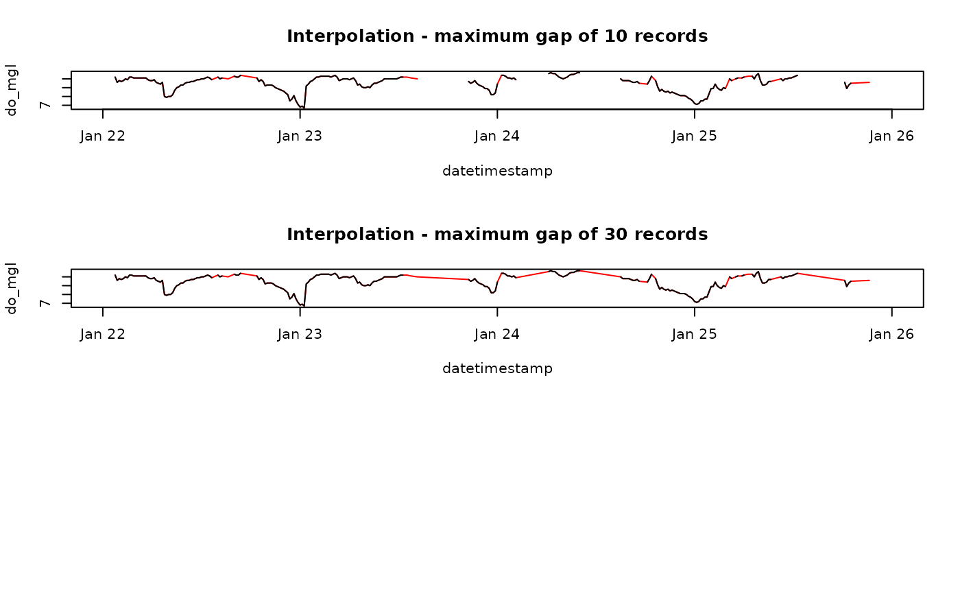
A common approach for handling missing data in time series analysis is linear interpolation. A simple curve fitting method is used to create a continuous set of records between observations separated by missing data. A required argument for the function is maxgap which defines the maximum gap size for interpolation. The ability of the interpolated data to approximate actual, unobserved trends is a function of the gap size. Interpolation between larger gaps are less likely to resemble patterns of an actual parameter, whereas interpolation between smaller gaps may be more likely to resemble actual patterns. An appropriate gap size limit depends on the unique characteristics of specific datasets or parameters.

See also

na.approx

Examples

data(apadbwq)
dat <- qaqc(apadbwq)
dat <- subset(dat, select = 'do_mgl', 
 subset = c('2013-01-22 00:00', '2013-01-26 00:00'))

# interpolate, maxgap of 10 records
fill1 <- na.approx(dat, params = 'do_mgl', maxgap = 10)

# interpolate maxgap of 30 records
fill2 <- na.approx(dat, params = 'do_mgl', maxgap = 30)

# plot for comparison
par(mfrow = c(3, 1))
plot(fill1, col = 'red', main = 'Interpolation - maximum gap of 10 records')
lines(dat)
plot(fill2, col = 'red', main = 'Interpolation - maximum gap of 30 records')
lines(dat)