Plot seasonal trends across all years

Plot seasonal trends by combining annual data

seasplot(dat_in, ...)

# S3 method for tidal
seasplot(
  dat_in,
  tau = NULL,
  predicted = TRUE,
  span = 0.4,
  lwd = 1,
  size = 2,
  alpha = 1,
  col_vec = NULL,
  grids = TRUE,
  logspace = TRUE,
  ...
)

# S3 method for tidalmean
seasplot(
  dat_in,
  predicted = TRUE,
  span = 0.4,
  lwd = 1,
  size = 2,
  alpha = 1,
  col_vec = NULL,
  grids = TRUE,
  logspace = TRUE,
  ...
)

Arguments

dat_in

Input data object

...

arguments passed to other methods

tau

numeric of quantile to plot

predicted

logical indicating if seasonal smooth is based on model predictions, default TRUE, otherwise the smooth is based on flow-normalized predictions

span

numeric indicating the smoothing parameter for the loess fit, passed to stat_smooth

lwd

numeric value indicating width of lines

size

numeric value indicating size of points

alpha

numeric value indicating transparency of points or lines

col_vec

chr string of plot colors to use, passed to gradcols. Any color palette from RColorBrewer can be used as a named input. Palettes from grDevices must be supplied as the returned string of colors for each palette.

grids

logical indicating if grid lines are present

logspace

logical indicating if plots are in log space

Details

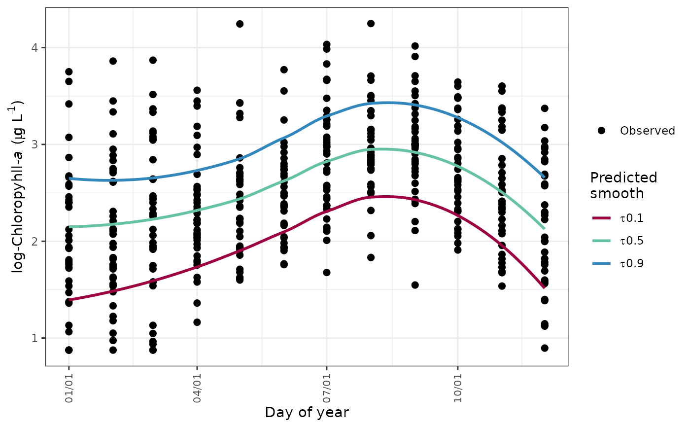
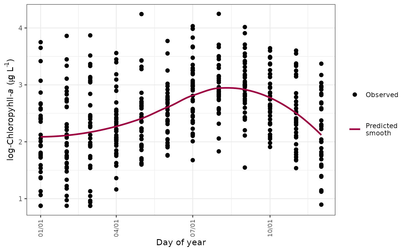
Seasonal variation across all years can be viewed by showing the observed annual data on a common y-axis. The year value is removed from the results such that the y-axis shows only the day of the year. A simple loess (locally estimated) polynomial smooth is added to show the seasonal trend in the results, where the smoother is fit through the model results for the observed data. The fit can be smoothed through the model predictions or the flow-normalized predictions, neither of which are shown on the plot.

See also

dynaplot, fitmoplot, gridplot, and sliceplot produce similar graphics except variation in the same month across years is emphasized.

Examples

# load a fitted tidal object
data(tidfit)

# plot using defaults
# defaults to all quantiles for tidal object
seasplot(tidfit)
#> `geom_smooth()` using method = 'loess' and formula = 'y ~ x'
#> Warning: Removed 10 rows containing non-finite values (`stat_smooth()`).


# tidalmean object
seasplot(tidfitmean)
#> `geom_smooth()` using method = 'loess' and formula = 'y ~ x'