Installation
This vignette provides an overview of the theory and use of the the Estuarine BAyesian Single-station Estimation (EBASE) R package for ecosystem metabolism. Use the following to install the package from R-Universe. The JAGS software must also be installed to use this package. Follow the instructions in the link to download and install the JAGS version appropriate for your operating system.
# Install EBASE in R:
install.packages('EBASE', repos = c('https://fawda123.r-universe.dev', 'https://cloud.r-project.org'))
Load the package after installation to use the functions.
Usage
An example file called exdat() is included with the
package that demonstrates the required time series format to use the
functions. It includes nearly a year of continuously monitored water
quality and meteorological data at the Apalachicola National Estuarine
Research Reserve. The required data include a date and time vector
(DateTimeStamp), dissolved oxygen (mg L-1,
DO_obs) , water temperature (C, Temp),
salinity (psu, Sal), PAR (W m-2, PAR), and
wind speed (m s-1, WSpd). The time step should be
consistent throughout the dataset and is indicated as an argument to the
ebase() function (see below). The exdat()
dataset can be viewed at any time after the package is loaded and is
used in the examples in the help files:
head(exdat)
#>         DateTimeStamp DO_obs Temp  Sal PAR WSpd
#> 1 2012-02-23 00:00:00    8.8 16.4 23.0   0  3.6
#> 2 2012-02-23 00:15:00    8.8 16.4 22.8   0  3.5
#> 3 2012-02-23 00:30:00    8.8 16.4 22.7   0  3.6
#> 4 2012-02-23 00:45:00    8.8 16.4 22.9   0  4.2
#> 5 2012-02-23 01:00:00    8.7 16.4 22.7   0  3.6
#> 6 2012-02-23 01:15:00    8.5 16.4 23.4   0  4.1
The core function to estimate metabolism is ebase(). The
metabolic estimates are based on a mass balance equation in Grace et al. (2015) with the gas exchange
estimate from Wanninkhof (2014). It is
similar to that provided by the BASEmetab R package at https://github.com/dgiling/BASEmetab, with modifications
to estimate different parameters optimized by the JAGS model:
More simply:
Net ecosystem metabolism (NEM) is then estimated as:
The metabolic estimates are defined by the change in dissolved oxygen over the time step , where gross production is provided by , respiration is provided by , and gas exchange is provided by the remainder. Required inputs for the equation are dissolved oxygen concentration as , solar radiation as , water column depth as (meters), and wind speed as . Other inputs for the schmidt number and dissolved oxygen at saturation are calculated from the observed data. The remaining three parameters , , and are estimated by likelihood given the observed data with the JAGS model using prior distributions shown in the model file. At each time step, the change in oxygen concentration between time steps is calculated from the equation using model inputs and parameter guesses, and then a finite difference approximation is used to estimate modeled oxygen concentration. The first modeled value starts at the mean oxygen concentration for all measurements in the optimization period. The estimated concentration is also returned at each time step, which can be compared to observed as one measure of model performance.
The following shows how to use the ebase() function with
a subset of four days from the exdat() example dataset.
Running the model on the entire year will take a few minutes, so a
subset is used:
library(dplyr)
library(lubridate)

# subset four days in June
dat <- exdat %>%
  filter(month(exdat$DateTimeStamp) == 6 & day(exdat$DateTimeStamp) %in% 1:4)

head(dat)
#>         DateTimeStamp DO_obs Temp  Sal PAR WSpd
#> 1 2012-06-01 00:00:00    4.5 29.5 23.0   0  2.0
#> 2 2012-06-01 00:15:00    5.1 29.5 23.3   0  2.3
#> 3 2012-06-01 00:30:00    4.8 29.5 23.4   0  2.1
#> 4 2012-06-01 00:45:00    4.8 29.5 23.3   0  2.0
#> 5 2012-06-01 01:00:00    4.8 29.5 23.1   0  1.7
#> 6 2012-06-01 01:15:00    5.0 29.5 24.0   0  1.8
Also note that any “dangling” observations at the start or end of the time series that do not include an entire day are removed from the input data prior to estimating metabolism. A warning is returned if these observations are found and removed.
res <- ebase(dat, interval = 900, Z = 1.85, n.chains = 2)
head(res)
#>         DateTimeStamp       Date grp    Z  DO_obs   DO_mod DO_modlo DO_modhi
#> 1 2012-06-01 00:00:00 2012-06-01   1 1.85 140.625 166.1132 166.1112 166.1152
#> 2 2012-06-01 00:15:00 2012-06-01   1 1.85 159.375 165.4135 165.1514 165.6797
#> 3 2012-06-01 00:30:00 2012-06-01   1 1.85 150.000 164.7458 164.2165 165.2784
#> 4 2012-06-01 00:45:00 2012-06-01   1 1.85 150.000 164.0582 163.2671 164.8557
#> 5 2012-06-01 01:00:00 2012-06-01   1 1.85 150.000 163.3622 162.3135 164.4221
#> 6 2012-06-01 01:15:00 2012-06-01   1 1.85 156.250 162.6401 161.3221 163.9645
#>         dDO converge       rsq        a       alo      ahi         b      blo
#> 1        NA     Fine 0.3316977       NA        NA       NA        NA       NA
#> 2 -67.17103     Fine 0.3316977 0.893719 0.5493333 1.237225 0.3099639 0.095399
#> 3 -64.09915     Fine 0.3316977 0.893719 0.5493333 1.237225 0.3099639 0.095399
#> 4 -66.01783     Fine 0.3316977 0.893719 0.5493333 1.237225 0.3099639 0.095399
#> 5 -66.81054     Fine 0.3316977 0.893719 0.5493333 1.237225 0.3099639 0.095399
#> 6 -69.32714     Fine 0.3316977 0.893719 0.5493333 1.237225 0.3099639 0.095399
#>         bhi  P Plo Phi        R      Rlo      Rhi       NEM     NEMlo     NEMhi
#> 1        NA NA  NA  NA       NA       NA       NA        NA        NA        NA
#> 2 0.4880948  0   0   0 141.3441 91.81687 189.3383 -141.3441 -189.3383 -91.81687
#> 3 0.4880948  0   0   0 141.3441 91.81687 189.3383 -141.3441 -189.3383 -91.81687
#> 4 0.4880948  0   0   0 141.3441 91.81687 189.3383 -141.3441 -189.3383 -91.81687
#> 5 0.4880948  0   0   0 141.3441 91.81687 189.3383 -141.3441 -189.3383 -91.81687
#> 6 0.4880948  0   0   0 141.3441 91.81687 189.3383 -141.3441 -189.3383 -91.81687
#>          D      Dlo      Dhi
#> 1       NA       NA       NA
#> 2 17.07768 5.256220 26.89167
#> 3 22.76066 7.016668 35.73653
#> 4 19.21110 5.935163 30.23677
#> 5 17.74459 5.472476 28.00036
#> 6 13.08888 4.054735 20.68587
The results are returned as a data frame with instantaneous metabolic
estimates for areal gross production (O2 mmol m-2 d-1, P or
from above as volumetric), respiration (O2 mmol m-2 d-1, R
from above as volumetric), and gas exchange (O2 mmol m-2 d-1,
D or the remainder of the equation from above as
volumetric, positive values as ingassing, negative values as
outgassing). NEM (net ecosystem metabolism, O2 mmol m-2
d-1) is also returned as P - R. Additional
parameters estimated by the model that are returned include
a and b as shown in the above equation. The
a parameter is a constant that represents the primary
production per quantum of light with units of (mmol m-2 d-1)/(W m-2) and
is used to estimate gross production (Grace et
al. 2015). The b parameter is a constant used to
estimate gas exchange in (cm hr-1)/(m2 s-2) (provided as 0.251 in eqn. 4
in Wanninkhof (2014)).
A plot of the results can be made with ebase_plot().
ebase_plot(res)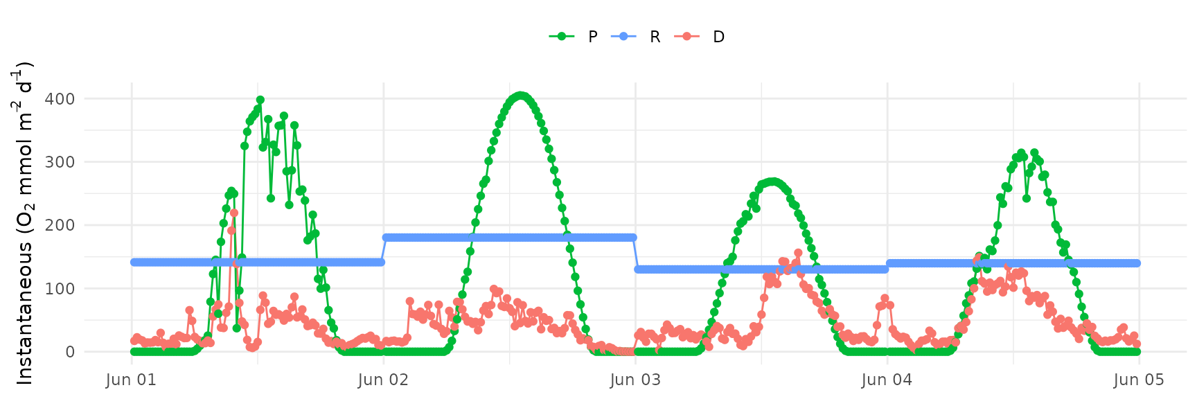
The daily averages can also be plotted by using
instantaneous = FALSE.
ebase_plot(res, instantaneous = FALSE)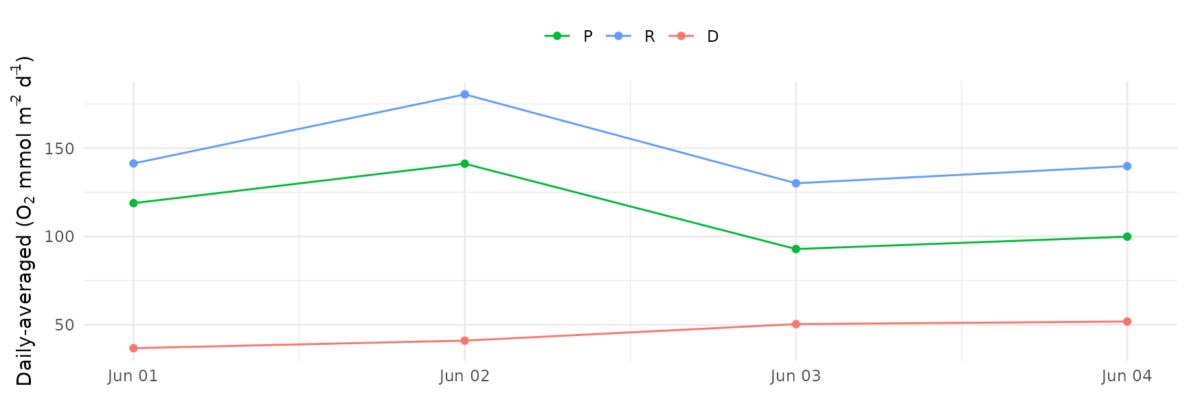
Similarly, a plot of net ecosystem metabolism (NEM) with production
and respiration can be made with ebase_plot() using
asnem = T. This plot shows NEM as the difference between
production and respiration. Gas exchange is not shown and respiration is
expressed negatively to show the negative contribution to NEM.
ebase_plot(res, asnem = T)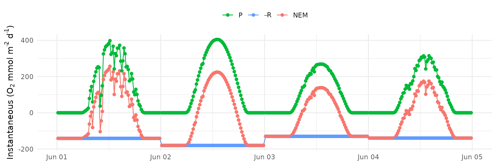
Execution time of the model can also be reduced by using multiple processors. This is done using doParrallel package and registering a parallel backend as below.
# setup parallel backend
library(doParallel)
cl <- makeCluster(2)
registerDoParallel(cl)

res <- ebase(dat, interval = 900, Z = 1.85, n.chains = 2)

stopCluster(cl)
Model fit can be assessed using the converge and
rsq columns from the returned results. The values in these
columns apply to each group in the grp column as specified
with the ndays argument. The converge column
indicates "Check convergence" or "Fine" if the
JAGS estimate converged at that iteration (repeated across rows for the
group). The n.chains argument can be increased if
convergence is not achieved. Similarly, the rsq column
shows the r-squared values of the linear fit between the modeled and
observed dissolved oxygen (repeated across rows for the group).
The model fit can also be assessed by comparing the observed and
modeled values for dissolved oxygen with the fit_plot()
function. Estimated values are shown as line and observed values are
shown as points.
fit_plot(res)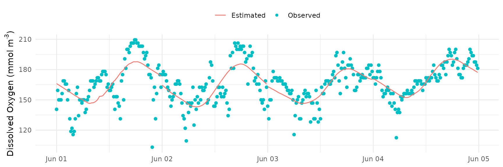
The comparison can also be separated by group with
bygroup = TRUE based on the value for the
ndays argument passed to ebase(). The
r-squared value of the fit between modeled and observed dissolved oxygen
is also shown in the facet label for the group.
fit_plot(res, bygroup = TRUE)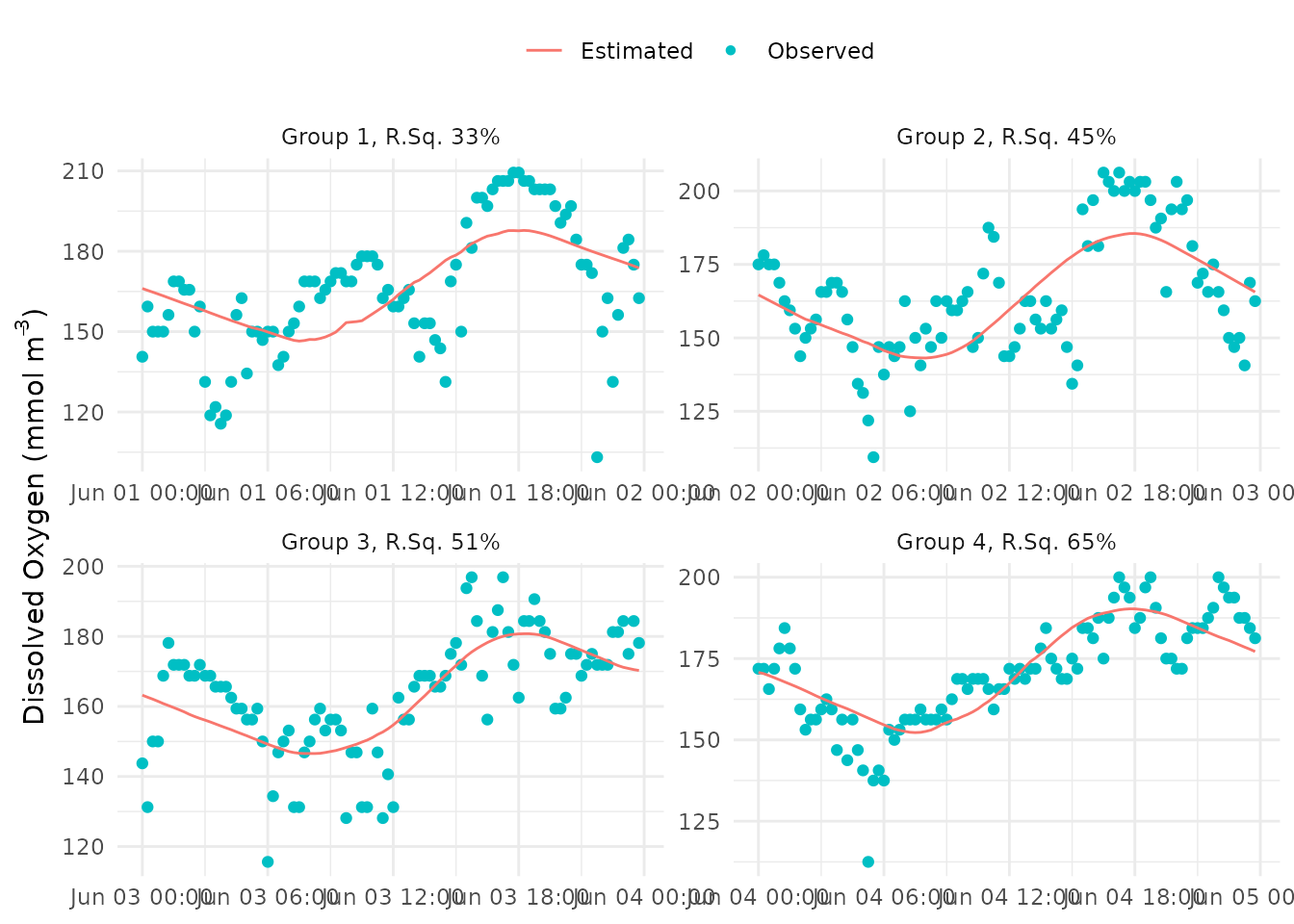
A scatterplot showing modeled versus observed dissolved oxygen can
also be returned by setting scatter = TRUE.
fit_plot(res, bygroup = TRUE, scatter = TRUE)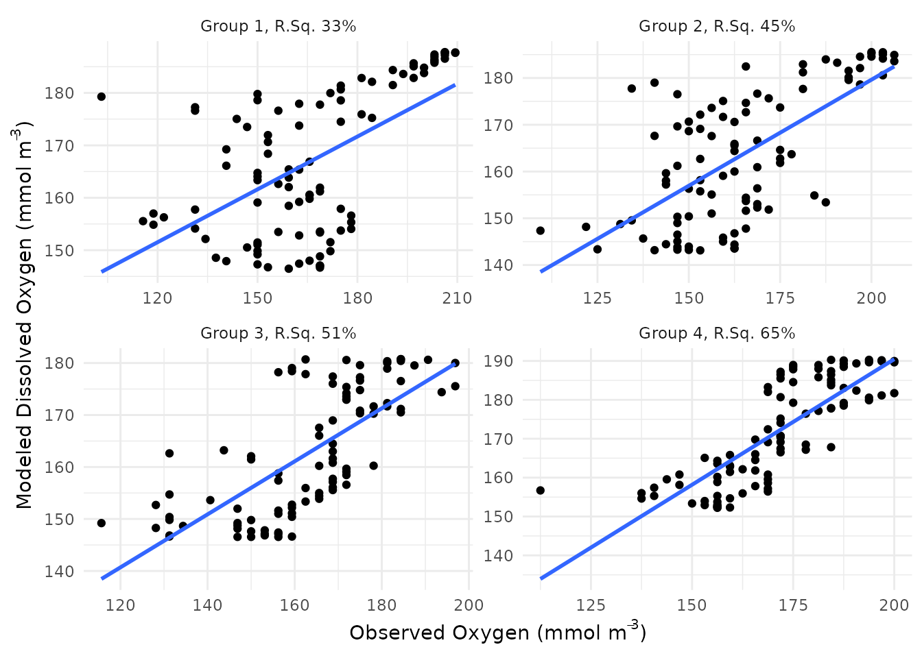
The prior distributions for the
,
,
and
parameters are defined in the model file included with the package as
normal Gaussian distributions with mean and standard deviations provided
by the aprior, rprior, and bprior
arguments in ebase(). The location of the model file can be
viewed as follows.
system.file('ebase_model.txt', package = 'EBASE')The default values for the priors were chosen based on the ability of
EBASE to reproduce known parameters from a forward metabolism model. An
additional constraint is that all the prior distributions are truncated
to be positive values as required by the core metabolism equation above.
The upper limit for
is also set as twice the default value of the mean in the
bprior argument. Units for each parameter are (mmol m-2
d-1)/(W m-2) for
,
mmol m-2 d-1 for
,
and (cm hr-1)/(m2 s-2) for
.
The prior distributions can be viewed with the
prior_plot() function. No changes are needed to the default
arguments for this function if the default arguments are used for
ebase(). The density curves are normalized such that the
peak value is always equal to 1.
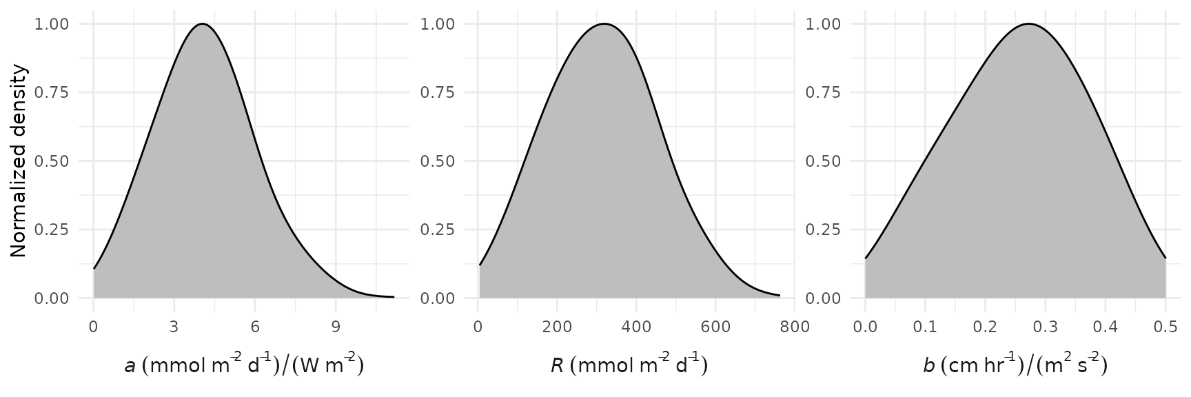
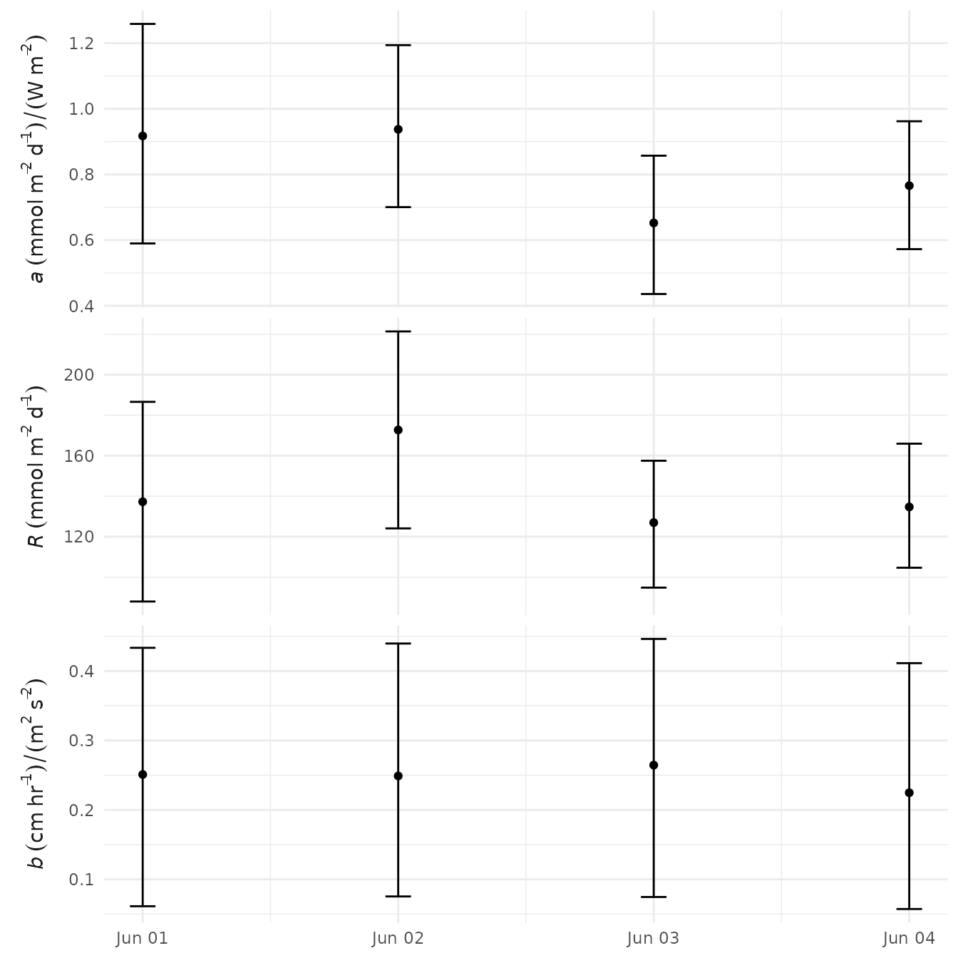
95% credible intervals for a, R (as areal),
and b are also returned with the output from
ebase() in the corresponding columns alo,
ahi, blo, bhi, Rlo,
and Rhi, for the 2.5th and 97.5th percentile estimates for
each parameter, respectively. These values indicate the interval within
which there is a 95% probability that the true parameter is in this
range and is a representation of the posterior distributions for each
parameter. Note that all values for these parameters are repeated across
rows, although only one estimate for each is returned based on the
number of days defined by ndays.
The credible intervals can be plotted with the
credible_plot() function.
credible_plot(res)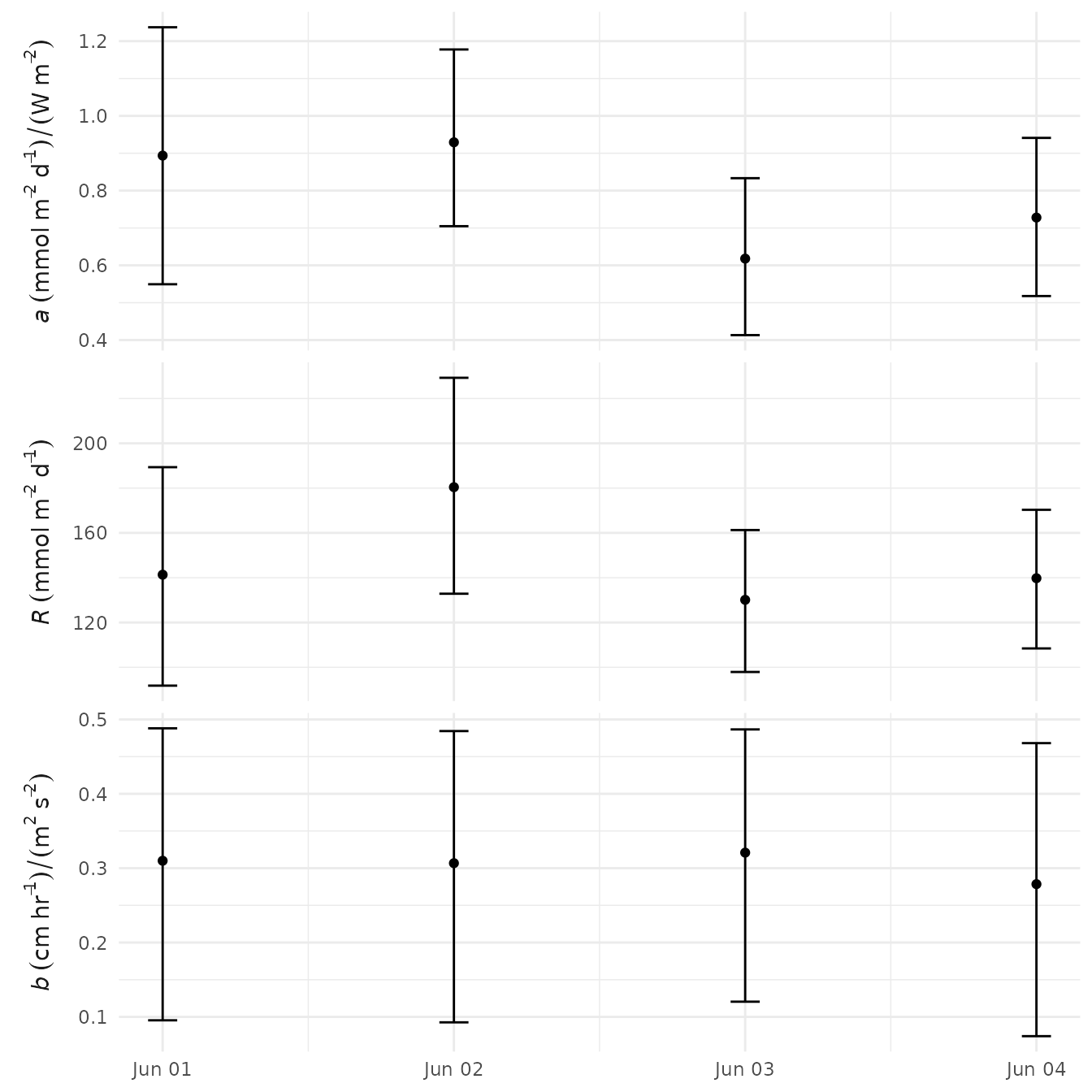
The credible intervals can also be retrieved as a data frame using
credible_prep(). This function is provided as a convenience
to parse the results from ebase().
credible_prep(res)
#> # A tibble: 12 × 6
#> # Groups:   grp [4]
#>    Date         grp var      mean       lo      hi
#>    <date>     <dbl> <fct>   <dbl>    <dbl>   <dbl>
#>  1 2012-06-01     1 a       0.894   0.549    1.24
#>  2 2012-06-01     1 R     141.     91.8    189.
#>  3 2012-06-01     1 b       0.310   0.0954   0.488
#>  4 2012-06-02     2 a       0.929   0.705    1.18
#>  5 2012-06-02     2 R     180.    133.     229.
#>  6 2012-06-02     2 b       0.307   0.0927   0.484
#>  7 2012-06-03     3 a       0.618   0.413    0.833
#>  8 2012-06-03     3 R     130.     97.9    161.
#>  9 2012-06-03     3 b       0.321   0.120    0.487
#> 10 2012-06-04     4 a       0.728   0.518    0.941
#> 11 2012-06-04     4 R     140.    108.     170.
#> 12 2012-06-04     4 b       0.279   0.0741   0.468
Finally, although ebase() can be used to estimate
metabolism for time series with several years of data, the
ebase_years() function can be used to estimate results
sequentially for each year. This is useful because model estimation
using ebase_years() will continue after a year fails, e.g.,
when some years have long periods of missing or erroneous data. This
eliminates the need to restart the model or further pre-process the
data. The same arguments for ebase() are used for
ebase_years(). Progress is printed directly in the console
and the user can specify the number of attempts for failed years before
proceeding to the following year.
Changing the default arguments
Equation optimization length
The ndays argument in ebase() defines the
model optimization period as the number of days that are used for
optimizing the above mass balance equation. By default, this is done
each day, i.e., ndays = 1 such that a loop is used that
applies the model equation to observations within each day, evaluated
iteratively from the first observation in a day to the last. Individual
parameter estimates for a, R, and
b are then returned for each day. However, more days can be
used to estimate the unknown parameters, such that the loop can be
evaluated for every ndays specified by the argument. The
ndays argument will separate the input data into groups of
consecutive days, where each group has a total number of days equal to
ndays. The final block may not include the complete number
of days specified by ndays if the number of unique dates in
the input data includes a remainder when divided by ndays,
e.g., if seven days are in the input data and ndays = 5,
there will be two groups where the first has five days and the second
has two days. The output data from ebase includes a column
that specifies the grouping that was used based on
ndays.
Here, the number of days used to optimize the equation is set to all days in the input data.
cl <- makeCluster(2)
registerDoParallel(cl)

res <- ebase(dat, interval = 900, Z = 1.85, n.chains = 2, ndays = 4)

stopCluster(cl)
And the resulting plot:
ebase_plot(res, instantaneous = TRUE)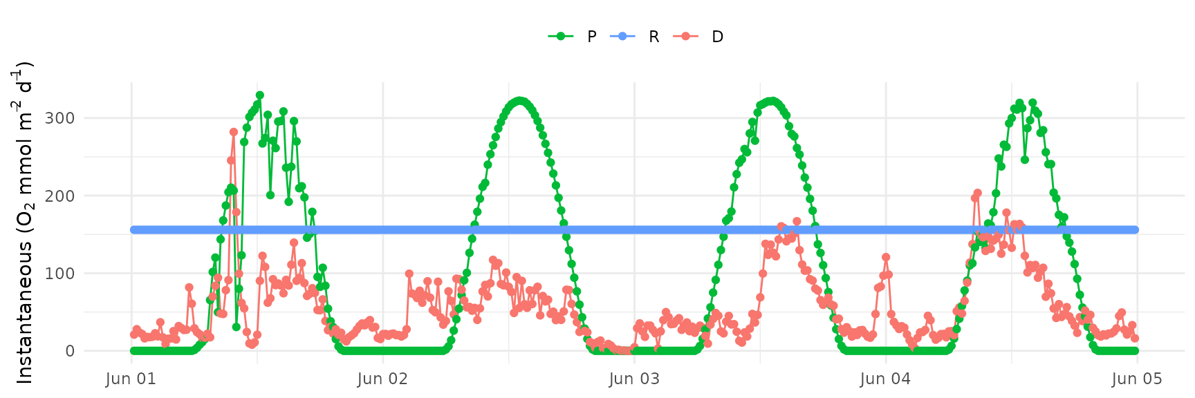
And the fit of observed and modeled dissolved oxygen (note the unbroken line for all days estimated together):
fit_plot(res)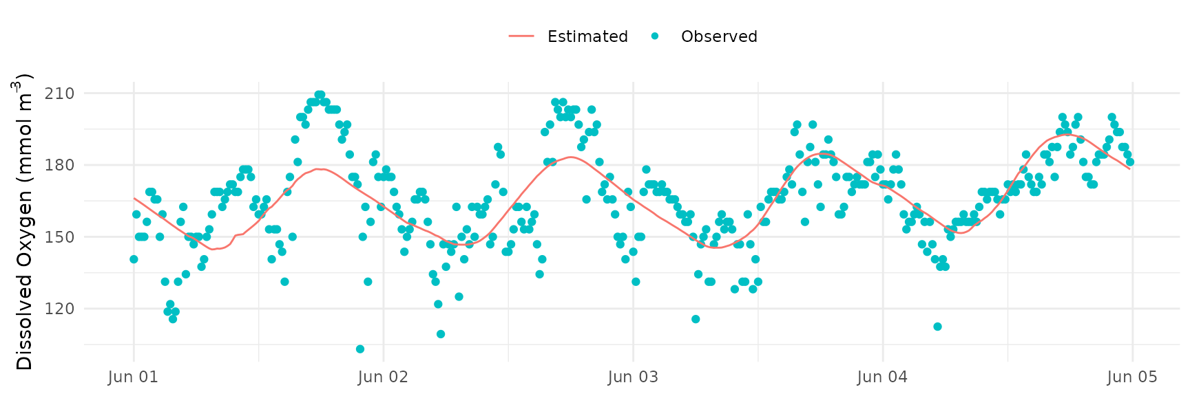
Starting value
The doave argument can be used to define which dissolved
oxygen value is used as the starting point in the Bayesian estimation
for the optimization period. The default setting
(doave = TRUE) will use the average of all the dissolved
oxygen values in the optimization period defined by ndays.
For example, the average of all dissolved oxygen values in each 24 hour
period will be used if doave = TRUE and
ndays = 1. The first dissolved oxygen observation of the
time series in the optimization period will be used as the starting
point if doave = F. In this case, the simulated dissolved
oxygen time series will always start at the first observed dissolved
oxygen value for each optimization period.
The default setting uses the average observed dissolved oxygen in
each optimization period as the starting value. Below,
doave = FALSE is used to set the first observed dissolved
oxygen as the starting value.
cl <- makeCluster(2)
registerDoParallel(cl)

res <- ebase(dat, interval = 900, Z = 1.85, n.chains = 2, ndays = 1, doave = F)

stopCluster(cl)
fit_plot(res)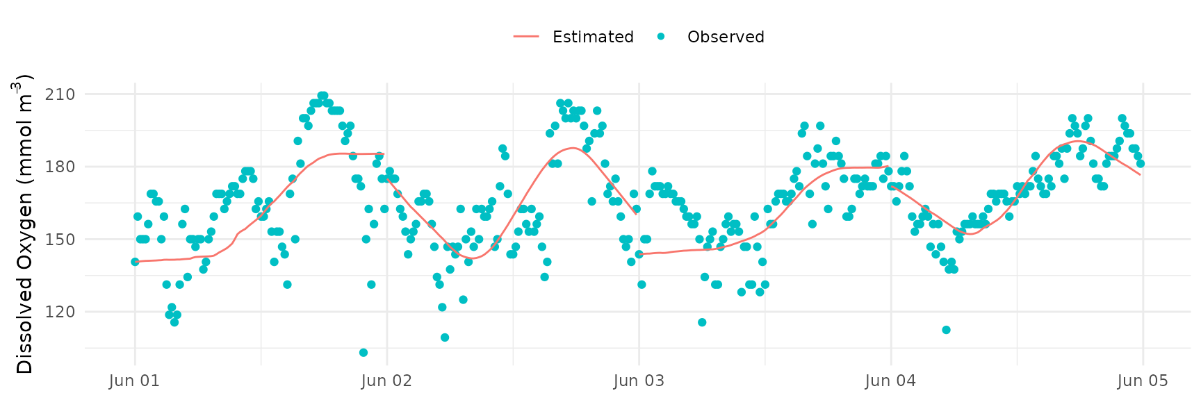
Missing values
Missing values in the input data for the specified time step in the
interval argument to ebase() must be
interpolated prior to estimating metabolism. It is the responsibility of
the user to verify that these interpolated values are not wildly
inaccurate. Missing values are linearly interpolated between non-missing
values at the time step specified by the value in interval.
This works well for small gaps, but can easily create inaccurate values
at gaps larger than a few hours.
As an example, the dat object above is subset to 90% of
its observations.
set.seed(222)
dat2 <- dat %>%
  slice_sample(prop = 0.9) %>%
  arrange(DateTimeStamp)
head(dat2)
#>         DateTimeStamp DO_obs Temp  Sal PAR WSpd
#> 1 2012-06-01 00:00:00    4.5 29.5 23.0   0  2.0
#> 2 2012-06-01 00:30:00    4.8 29.5 23.4   0  2.1
#> 3 2012-06-01 01:00:00    4.8 29.5 23.1   0  1.7
#> 4 2012-06-01 01:30:00    5.4 29.6 24.9   0  1.8
#> 5 2012-06-01 01:45:00    5.4 29.6 24.6   0  1.8
#> 6 2012-06-01 02:00:00    5.3 29.6 24.8   0  2.0
The ebase_prep() function is used internally to
ebase to prepare the data for the metabolism calculations.
This function interpolates the missing data and returns a column
isinterp that specifies TRUE or
FALSE if a value is interpolated.
dat2interp <- ebase_prep(dat2, Z = 1.85, interval = 900)
head(dat2interp)
#>         Date       DateTimeStamp isinterp  DO_obs   DO_sat    Z Temp  Sal PAR
#> 1 2012-06-02 2012-06-02 00:00:00    FALSE 175.000 213.4922 1.85 28.8 21.8   0
#> 2 2012-06-02 2012-06-02 00:15:00    FALSE 178.125 212.6648 1.85 28.8 22.5   0
#> 3 2012-06-02 2012-06-02 00:30:00    FALSE 175.000 211.7234 1.85 28.9 23.0   0
#> 4 2012-06-02 2012-06-02 00:45:00    FALSE 175.000 212.3111 1.85 28.9 22.5   0
#> 5 2012-06-02 2012-06-02 01:00:00    FALSE 168.750 212.1933 1.85 29.0 22.3   0
#> 6 2012-06-02 2012-06-02 01:15:00    FALSE 162.500 211.7237 1.85 29.0 22.7   0
#>   WSpd       sc grp
#> 1  1.9 355.5996   1
#> 2  1.8 356.3840   1
#> 3  1.9 355.2102   1
#> 4  1.9 354.6523   1
#> 5  1.8 352.7068   1
#> 6  1.8 353.1511   1
The interpolated values can be visually inspected using the
interp_plot() function.
interp_plot(dat2, Z = 1.85, interval = 900, param = 'DO_sat')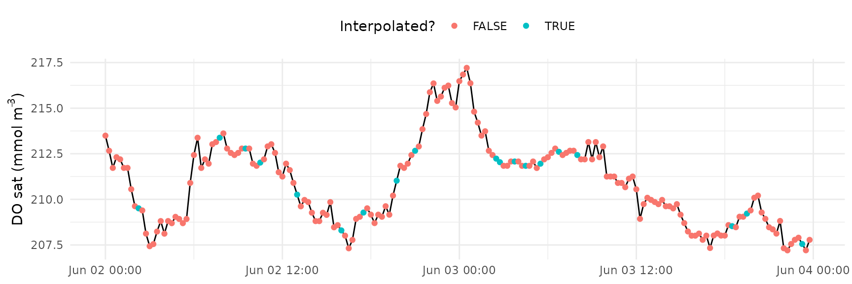
The ebase() function includes the maxinterp
argument to assign NA values to continuously interpolated
rows with length greater than the value defined by
maxinterp. This value is set to 12 hours by default and
applies to the groupings defined by ndays, i.e., any group
with a continuous set of interpolated values where the time is greater
than 12 hours are assigned NA (except Date and
DateTimeStamp). The numeric value passed to
maxinterp is the number of time steps for the input data,
e.g., 48 would be 12 hours if the time step is 900 seconds.
Changing priors
If the default values prior distributions are changed for
ebase(), the prior_plot() function can be used
to assess how changing characteristics of the prior distributions could
influence the resulting parameter estimates and their posterior
distributions (e.g., as shown with credible_plot()).
Here, the prior distribution for the parameter is changed to have a mean of 0.4 and standard deviation of 1.
prior_plot(bprior = c(0.2, 0.1))
The same change to the prior distribution for the
parameter is applied to ebase()
cl <- makeCluster(2)
registerDoParallel(cl)

res <- ebase(dat, interval = 900, Z = 1.85, n.chains = 2, bprior = c(0.2, 0.1))

stopCluster(cl)

ebase_plot(res, instantaneous = TRUE)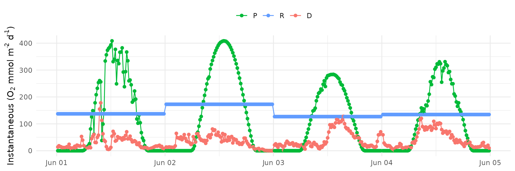
The credible_plot() function can be used to assess how
changing the prior distributions has an influence on the posterior
distributions of the parameters.
credible_plot(res)